8. PIMPLE Predictor–Corrector Method

PIMPLE combines a SIMPLE-family nonlinear outer iteration with PISO-style pressure–momentum correctors. The outer iteration refreshes the nonlinear transport coefficients and coupled physical state. The corrector stages then reduce the remaining continuity and momentum-splitting error without repeating every implicit transport solve.

The Stream formulation was developed from the operator-splitting construction used by PISO [Iss86, TW04], combined with a time-consistent momentum-interpolation treatment [Pas11]. Its original development and validation are documented in the project final report [TW21].

This chapter uses the finite-volume and pressure-correction machinery already developed in:

• Chapter 4 for assembled transport rows;

• Chapter 5 for the cell-to-face momentum response; and

• Chapter 6 for the compressible pressure-correction equation.

The detailed balances below use a stationary mesh, no mass sources, and first-order backward differencing (BDF1). The pressure-stage construction also applies to other time discretizations when their storage coefficients and known history terms are retained consistently.

8.1. Iteration Hierarchy

The indices distinguish physical time from the iterations within one time step:

Index	Role
\(n\)	Accepted physical-time level; the step advances to \(n+1\)
\(k\)	Nonlinear outer iteration, including implicit predictor solves
\(m=0,\ldots,N_c-1\)	PISO corrector, taking state \(m\) to \(m+1\)
\(j=0,\ldots,J-1\)	Deferred pressure stage; \(J\ge1\) is the number of stages per corrector
\(\ell\)	Linear iteration within any predictor or corrector equation solve

Figure 8.1.1 compares the two loop structures. The physical time step stays fixed while the PIMPLE outer iteration repeats.

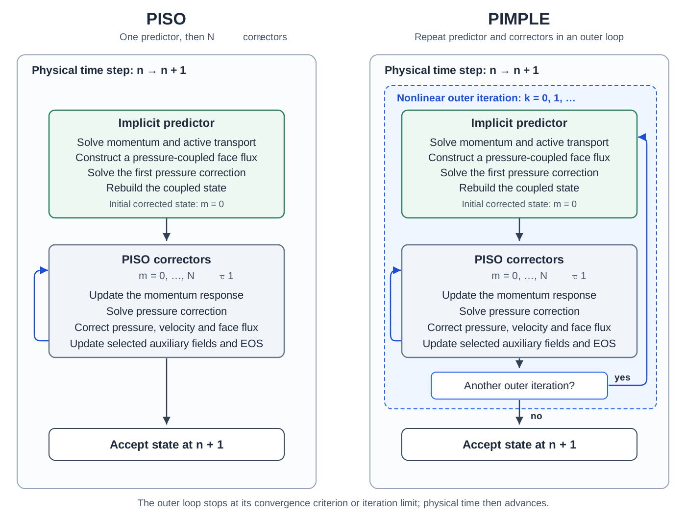
Fig. 8.1.1 One physical time step of PISO and PIMPLE. Each predictor includes the initial pressure correction; \(N_c\) subsequent correctors update the coupled state. PIMPLE repeats the sequence through outer iteration \(k\) until its convergence criterion or iteration limit is reached. Internal linear-solver and additional pressure-correction stages are omitted.

The pressure stages \(j\) and linear iterations \(\ell\) are shown in Figure 8.1.2.

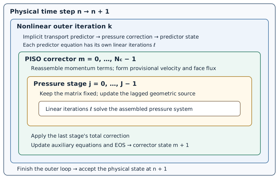
Fig. 8.1.2 Nested PIMPLE iterations. Linear solves occur in the predictor and in each pressure stage. The final pressure stage supplies the correction used to complete one PISO corrector.

For one physical time step, the state sequence is

(8.1.1)\[\boldsymbol{Q}^{n} \longrightarrow \boldsymbol{Q}^{n+1,k,0} \longrightarrow \boldsymbol{Q}^{n+1,k,1} \longrightarrow\cdots\longrightarrow \boldsymbol{Q}^{n+1,k,N_c} \longrightarrow \boldsymbol{Q}^{n+1,k+1,0}\]

Here \(\boldsymbol{Q}^{n+1,k,0}\) is the state after the implicit predictor and its first pressure correction, and \(N_c\) is the number of PISO correctors. Once the outer convergence or iteration criterion is satisfied, \(\boldsymbol{Q}^{n+1}\) is accepted from the last outer state.

8.2. Implicit Predictor

The physical-time index \(n+1\) is suppressed on provisional fields. At outer iteration \(k\), freeze the current nonlinear coefficients and write the time-discrete momentum row for cell \(P\) as

(8.2.1)\[{}^{(u)}\!a_P^{k}\vec{u}_P^{*,k} = \sum_{N\in\mathcal{N}(P)} {}^{(u)}\!a_{P,N}^{k}\vec{u}_N^{*,k} +{}^{(u)}\!\vec{b}_P^{k} +\vec{b}_{P,t}^{n} -\mathcal{G}_P\!\left(p^{k}\right)\]

Here \({}^{(u)}\!a_P^{k}\) contains the spatial and implicit temporal diagonal, \({}^{(u)}\!\vec{b}_P^{k}\) contains explicit spatial and physical-source terms, and \(\vec{b}_{P,t}^{n}\) contains known time-history terms. The discrete pressure force uses the stored face area vector \(\vec A_f\) and the incidence sign \(\sigma_{Pf}\) from Loci Face Orientation and Cell Incidence:

(8.2.2)\[\mathcal{G}_P(p) = \sum_{f\in\mathcal{F}(P)} \sigma_{Pf}p_f\vec{A}_f \simeq \Omega_P\nabla p_P\]

Define the non-pressure momentum source

(8.2.3)\[\vec{H}_P^{k}(\vec{u}) = \sum_N {}^{(u)}\!a_{P,N}^{k}\vec{u}_N +{}^{(u)}\!\vec{b}_P^{k} +\vec{b}_{P,t}^{n}\]

The predictor row then exposes the two pieces needed by pressure correction:

(8.2.4)\[\vec{u}_P^{*,k} = \frac{\vec{H}_P^{k}(\vec{u}^{*,k})}{{}^{(u)}\!a_P^{k}} - \frac{\mathcal{G}_P(p^k)}{{}^{(u)}\!a_P^{k}}\]

The momentum equation is solved implicitly at this stage. The selected thermal, turbulence, species, phase, and other active predictor equations are likewise solved within the outer iteration before the complete predictor state enters the corrector loop.

8.2.1. Temporal Diagonal Split

The face flux must retain the same temporal response as the cell momentum equation. Split the momentum diagonal into non-temporal and leading temporal parts,

(8.2.1.1)\[{}^{(u)}\!a_P^{k} = {}^{(u)}\!\widetilde a_P^{k}+c_{0,P}^{k} = {}^{(u)}\!\widetilde a_P^{k}\left(1+\delta_P^k\right) \qquad \delta_P^k=\frac{c_{0,P}^{k}}{{}^{(u)}\!\widetilde a_P^{k}}\]

Here \(c_{0,P}^{k}\) is the temporal contribution actually retained in the momentum diagonal. In the continuity-subtracted BDF1 row of Eq. (5.5.2), it is \(\rho_P^n\Omega_P/\Delta t\). The diagonal split and its history terms must belong to the same momentum-row form.

Scope of the Temporal Ratios

The ratios below require nonzero non-temporal diagonals and nonzero cell and face denominators. If a non-temporal diagonal vanishes, the ratio form is undefined even when the complete momentum diagonal is finite and nonzero. The cell update can still be written using the complete diagonal in Eq. (8.3.6); the face formula requires a separately derived limit or interpolation using complete diagonals.

Multistep and Crank–Nicolson formulas must carry their corresponding history and spatial weights into both cell and face equations. The additional terms are developed in Time-Consistent Momentum Interpolation and Higher-Order Temporal Integration and Splitting; changing \(c_{0,P}^{k}\) alone does not produce those extensions.

8.2.2. Predictor Face Flux

For a local two-cell face relation, set \(P=\operatorname{cl}(f)\) and \(N=\operatorname{cr}(f)\). The stored area vector points from \(P\) to \(N\). Define the volumetric and mass fluxes on the stationary mesh by

(8.2.2.1)\[\mathcal{V}_f=\vec{u}_f\cdot\vec{A}_f \qquad \dot m_f=\rho_f\mathcal{V}_f\]

Momentum-weighted interpolation converts Eq. (8.2.4) into a pressure-sensitive face flux. Its predictor form can be written

(8.2.2.2)\[\dot m_f^{*,k} = \widehat{\dot m}_f^{k} -d_f^{k}\left(p_N^k-p_P^k\right) \qquad d_f^{k}>0\]

The term \(\widehat{\dot m}_f^{k}\) contains the interpolated non-pressure momentum contribution, temporal history, and explicit geometry terms. Holding that term and the interpolation coefficients fixed gives \(\partial\dot m_f^{*,k}/\partial(p_N^k-p_P^k)=-d_f^k\). Thus, \(d_f^k>0\) is the magnitude of this direct mass-flux sensitivity. The pressure-correction coefficient also depends on the selected SIMPLE-family approximation to the cell-velocity change, as derived in Connection to the Pressure-Correction Equation.

8.2.3. Predictor Pressure Correction

The predicted flux generally does not satisfy continuity. Define its cell residual by

(8.2.3.1)\[R_P^{*,k} = \frac{\Omega_P}{\Delta t}\left(\rho_P^k-\rho_P^n\right) +\sum_{f\in\mathcal{F}(P)}\sigma_{Pf}\dot m_f^{*,k}\]

The density \(\rho_P^n\) belongs to the accepted time level. Introduce the predictor pressure correction \(p_P^{\prime,*,k}\). For the direct pressure-difference contribution, the face response is

(8.2.3.2)\[\dot m_f^{\prime,*,k} = -d_f^{k}\left(p_N^{\prime,*,k}-p_P^{\prime,*,k}\right) +\dot m_{f,\rho}^{\prime,*,k}\]

For compressible flow, the acoustic tangent supplies

(8.2.3.3)\[\rho_P^{\prime,*,k} \approx \left(\frac{\partial\rho}{\partial p}\right)_{s,Y}^{k} p_P^{\prime,*,k} = \frac{p_P^{\prime,*,k}}{a_{s,P}^{2}}\]

The term \(\dot m_{f,\rho}^{\prime,*,k}\) carries the upwind face density correction with the provisional volumetric flux. Substitution into continuity gives the standard row

(8.2.3.4)\[{}^{(p')}\!a_P^{*,k}p_P^{\prime,*,k} = \sum_N {}^{(p')}\!a_{P,N}^{*,k}p_N^{\prime,*,k} +{}^{(p')}\!b_P^{*,k}\]

The detailed acoustic, boundary, and face-coefficient contributions are those derived in Chapter 6.

After solving Eq. (8.2.3.4), the predictor state that enters the PISO loop is

(8.2.3.5)\[\begin{split}p_P^{k,0} &=p_P^k+\alpha_p p_P^{\prime,*,k}\\ \vec{u}_P^{k,0} &=\vec{u}_P^{*,k}+\vec{u}_P^{\prime,*,k}\\ \dot m_f^{k,0} &=\dot m_f^{*,k}+\dot m_f^{\prime,*,k}\end{split}\]

The outer predictor may use the SIMPLE or SIMPLEC response described in Chapter 7. Each subsequent PISO corrector uses the unrelaxed momentum response. It updates the state produced by the predictor without repeating the under-relaxed outer iteration.

Predictor-Stage Result

The implicit transport solves, pressure correction, flux correction, and EOS closure together produce the complete state

(8.2.3.6)\[\boldsymbol{Q}^{n+1,k,0} = \left\{ p^{k,0},\vec{u}^{\,k,0},\mathcal{V}_f^{k,0}, \Theta^{k,0},\boldsymbol{Y}^{k,0},\rho^{k,0},\ldots \right\}\]

This state supplies the incoming fields and coefficients for the first PISO corrector.

8.3. PISO Corrector Derivation

The first corrector is initialized from the complete predictor-stage state:

(8.3.1)\[p^0=p^{k,0} \qquad \vec{u}^{\,0}=\vec{u}^{\,k,0} \qquad \mathcal{V}_f^0=\mathcal{V}_f^{k,0} \qquad \boldsymbol{Q}^0=\boldsymbol{Q}^{n+1,k,0}\]

Within this outer iteration, suppress \(k\) and denote the incoming fields for corrector \(m\) by superscript \(m\). The latest face flux and thermodynamic state determine a newly assembled momentum diagonal, while the incoming velocity supplies the neighbor values in the corresponding non-pressure momentum contribution. Denote saved incoming quantities by superscript \(o\) and the newly assembled corrector quantities by superscript \(c\):

(8.3.2)\[\begin{split}{}^{(u)}\!a_P^{o}\vec{u}_P^{m} &= \vec{H}_P^{o}-\mathcal{G}_P(p^m)\\ {}^{(u)}\!a_P^{c}\vec{u}_P^{m+1} &= \vec{H}_P^{c}-\mathcal{G}_P(p^{m+1})\end{split}\]

The corrector quantities have the schematic dependencies

(8.3.3)\[\begin{split}{}^{(u)}\!a_P^{c} &= \mathcal{A}_P\!\left(\mathcal{V}^{m},\boldsymbol{Q}^{m}\right)\\ \vec{H}_P^{c} &= \sum_N {}^{(u)}\!a_{P,N}^{c}\vec{u}_N^{m} +{}^{(u)}\!\vec{b}_P^{c} +\vec{b}_{P,t}^{n}\end{split}\]

Here \(\mathcal{A}_P\) denotes assembly of the momentum diagonal from the latest face flux, properties, and source linearizations. Thus, the corrector refreshes the momentum response using the latest state but remains explicit in the velocity update.

Define the total pressure correction by

(8.3.4)\[p^{m+1}=p^m+p^{\prime,m}\]

Subtract the first row in Eq. (8.3.2) from the second:

(8.3.5)\[{}^{(u)}\!a_P^{c}\vec{u}_P^{m+1} -{}^{(u)}\!a_P^{o}\vec{u}_P^{m} = \left(\vec{H}_P^{c}-\vec{H}_P^{o}\right) -\mathcal{G}_P(p^{\prime,m})\]

Solving for the corrected velocity gives

(8.3.6)\[\vec{u}_P^{m+1} = \frac{{}^{(u)}\!a_P^{o}}{{}^{(u)}\!a_P^{c}}\vec{u}_P^{m} +\frac{\vec{H}_P^{c}-\vec{H}_P^{o}}{{}^{(u)}\!a_P^{c}} -\frac{\mathcal{G}_P(p^{\prime,m})}{{}^{(u)}\!a_P^{c}}\]

Equation (8.3.6) separates three effects: the change in the diagonal, the change in the explicit momentum source, and the new pressure correction.

8.3.1. Timestep-Consistent Hatted Velocity

Apply the temporal split of Eq. (8.2.1.1) to both corrector states and define

(8.3.1.1)\[\widehat{\vec{u}}_P^{m} = \frac{\vec{H}_P^{c}-\vec{H}_P^{o}} {{}^{(u)}\!\widetilde a_P^{c}}\]

Equation (8.3.6) becomes

(8.3.1.2)\[\vec{u}_P^{m+1} = \frac{1+\delta_P^{o}}{1+\delta_P^{c}} \frac{{}^{(u)}\!\widetilde a_P^{o}}{{}^{(u)}\!\widetilde a_P^{c}} \vec{u}_P^{m} +\frac{\widehat{\vec{u}}_P^{m}}{1+\delta_P^{c}} -\frac{\mathcal{G}_P(p^{\prime,m})} {{}^{(u)}\!\widetilde a_P^{c}(1+\delta_P^{c})}\]

The temporal factor is now explicit and can be carried consistently to the face. For an interior face between \(P\) and \(N\), let \(w_P+w_N=1\) denote the cell-to-face interpolation weights. Interpolate the old and current temporal ratios, the non-temporal diagonal ratio, and the hatted cell velocity as

(8.3.1.3)\[\begin{split}\delta_f^{o}=w_P\delta_P^o+w_N\delta_N^o \qquad \delta_f^{c}=w_P\delta_P^c+w_N\delta_N^c \\ r_{a,f} = w_P\frac{{}^{(u)}\!\widetilde a_P^{o}}{{}^{(u)}\!\widetilde a_P^{c}} +w_N\frac{{}^{(u)}\!\widetilde a_N^{o}}{{}^{(u)}\!\widetilde a_N^{c}} \qquad \widehat{\vec{u}}_f^{m} = w_P\widehat{\vec{u}}_P^{m} +w_N\widehat{\vec{u}}_N^{m}\end{split}\]

Approximate the face update by interpolating these factors separately and using the incoming face flux for the term multiplying the diagonal ratios:

(8.3.1.4)\[\widehat{\mathcal{V}}_f^{m} = \frac{(1+\delta_f^o)r_{a,f}}{1+\delta_f^c} \mathcal{V}_f^{m} + \frac{\widehat{\vec{u}}_f^{m}\cdot\vec{A}_f} {1+\delta_f^c}\]

Equation (8.3.1.4) defines the provisional face flux. Separate interpolation of the factors is a face approximation; it is not an exact interpolation of their cellwise products. The pressure correction supplies the remaining normal pressure-gradient contribution.

8.3.2. Corrector Pressure Response

For the time-consistent form, the interior-face mass-flux coefficient is

(8.3.2.1)\[d_f^{m} = \rho_f A_f \frac{ \mathcal{I}_f\!\left(\dfrac{\Omega}{{}^{(u)}\!\widetilde a^{c}}\right) }{ (1+\delta_f^c)\ell_f }\]

The projected cell-center spacing \(\ell_f\) is defined in Eq. (5.3.3.4). The PISO corrector uses the unrelaxed momentum diagonal, so its pressure coefficient contains no momentum under-relaxation factor.

For the geometric reconstruction, label the stored left and right cells \(L=\operatorname{cl}(f)\) and \(R=\operatorname{cr}(f)\). Let \(\vec x_f\) be the face centroid, \(\vec x_L,\vec x_R\) the cell centers, and \(\hat{\vec n}_f=\vec A_f/A_f\). The transverse offsets from each cell center to the face-normal line through \(\vec x_f\) are

(8.3.2.2)\[\begin{split}\vec s_{L,f} &=\vec x_f-\vec x_L -\bigl[(\vec x_f-\vec x_L)\cdot\hat{\vec n}_f\bigr]\hat{\vec n}_f \\ \vec s_{R,f} &=\vec x_f-\vec x_R -\bigl[(\vec x_f-\vec x_R)\cdot\hat{\vec n}_f\bigr]\hat{\vec n}_f\end{split}\]

For a scalar pressure field \(q\), extrapolate from each cell center along these offsets. Their difference defines the geometric pressure correction:

(8.3.2.3)\[\begin{split}\mathcal E_f(q) &=\nabla q_L\cdot\vec s_{L,f}-\nabla q_R\cdot\vec s_{R,f} \\ \left(\frac{\partial q}{\partial n}\right)_f &\approx\frac{q_R-q_L-\mathcal E_f(q)}{\ell_f}\end{split}\]

For a linear field with exact cell gradients, this gives the exact normal derivative and agrees with Eq. (5.3.6.2). For a general field, the two reconstructed cell gradients define the extrapolation.

At corrector \(m\), hold the provisional velocity and face flux, density, acoustic tangent, and pressure coefficients fixed. Start the \(J\) pressure stages with \(p^{\prime,m,-1}=0\); the index \(-1\) denotes the initial zero geometric correction. At stage \(j=0,\ldots,J-1\), evaluate the transverse term using the preceding stage and solve for the current two-cell pressure difference. The volume-flux correction is

(8.3.2.4)\[\mathcal V_f^{\prime,m,j} =-\frac{d_f^m}{\rho_f} \left(p_R^{\prime,m,j}-p_L^{\prime,m,j}\right) +\frac{d_f^m}{\rho_f}\mathcal E_f(p^{\prime,m,j-1})\]

Linearize \(\dot m_f=\rho_f\mathcal V_f\) about the provisional flux and drop the product of density and volume-flux corrections:

(8.3.2.5)\[\begin{split}\dot m_f^{\prime,m,j} &=\rho_f\mathcal V_f^{\prime,m,j} +\widehat{\mathcal V}_f^m\rho_{\mathrm{up}}^{\prime,m,j} \\ \rho_P^{\prime,m,j}&=\psi_P^m p_P^{\prime,m,j} \qquad \psi_P^m=\frac{1}{(a_{s,P}^m)^2}\end{split}\]

The upwind cell is selected by the sign of the fixed \(\widehat{\mathcal V}_f^m\). The acoustic density term enters the linearized mass balance; the volume-flux update uses Eq. (8.3.2.4). For constant-density flow, set \(\psi=0\) and omit the density correction.

8.3.3. Pressure Stages in the Cell Balance

The provisional BDF1 continuity residual includes both the density inventory and the signed sum of hatted mass fluxes:

(8.3.3.1)\[\begin{split}\widehat R_P^m &=\frac{\Omega_P}{\Delta t}(\rho_P^m-\rho_P^n) +\sum_{f\in\mathcal F(P)}\sigma_{Pf}\widehat{\dot m}_f^m \\ \widehat{\dot m}_f^m&=\rho_f\widehat{\mathcal V}_f^m\end{split}\]

On a prescribed-flux boundary, use the imposed mass flux in this residual. Linearizing continuity about the same provisional state gives

(8.3.3.2)\[\frac{\Omega_P\psi_P^m}{\Delta t}p_P^{\prime,m,j} +\sum_{f\in\mathcal F(P)}\sigma_{Pf}\dot m_f^{\prime,m,j} =-\widehat R_P^m\]

The residual \(\widehat R_P^m\) contains the complete BDF1 time history. To collect the interior-face coefficients, let \(\mathcal F_P^{\mathrm{int}}\) be the internal faces incident on \(P\), and let \(N_f(P)\) be the cell across face \(f\). For an internal face, \(\sigma_{Pf}(p_L'-p_R')=p_P'-p_{N_f(P)}'\). For a cell whose faces are internal or have prescribed mass flux, the boundary mass-flux corrections vanish. Substitute the two flux corrections into the linearized balance and move the lagged geometric term to the RHS:

(8.3.3.3)\[\begin{split}\frac{\Omega_P\psi_P^m}{\Delta t}p_P^{\prime,m,j} &+\sum_{f\in\mathcal F_P^{\mathrm{int}}} d_f^m(p_P^{\prime,m,j}-p_{N_f(P)}^{\prime,m,j}) \\ &+\sum_{f\in\mathcal F_P^{\mathrm{int}}} \sigma_{Pf}\widehat{\mathcal V}_f^m \psi_{\mathrm{up}}^m p_{\mathrm{up}}^{\prime,m,j} \\ &=-\widehat R_P^m -\sum_{f\in\mathcal F_P^{\mathrm{int}}} \sigma_{Pf}d_f^m\mathcal E_f(p^{\prime,m,j-1})\end{split}\]

A pressure-responsive boundary supplies its one-sided pressure and acoustic terms, using the boundary relations in Pressure-Correction Equation on Unstructured Grids.

Corrector Pressure System

Collecting the unknowns gives

(8.3.3.4)\[{}^{(p')}\!a_P^m p_P^{\prime,m,j} =\sum_N{}^{(p')}\!a_{P,N}^m p_N^{\prime,m,j} +{}^{(p')}\!b_P^{m,j}\]

For the internal and prescribed-flux faces just considered,

(8.3.3.5)\[\begin{split}{}^{(p')}\!a_P^m &=\frac{\Omega_P\psi_P^m}{\Delta t} +\sum_{f\in\mathcal F_P^{\mathrm{int}}} \left[d_f^m+\max(\sigma_{Pf}\widehat{\mathcal V}_f^m,0)\psi_P^m\right] \\ {}^{(p')}\!a_{P,N}^m &=\sum_{\substack{f\in\mathcal F_P^{\mathrm{int}}\\N_f(P)=N}} \left[d_f^m+\max(-\sigma_{Pf}\widehat{\mathcal V}_f^m,0)\psi_N^m\right] \\ {}^{(p')}\!b_P^{m,j} &=-\widehat R_P^m -\sum_{f\in\mathcal F_P^{\mathrm{int}}} \sigma_{Pf}d_f^m\mathcal E_f(p^{\prime,m,j-1})\end{split}\]

The matrix and \(\widehat R_P^m\) are independent of \(j\). Each stage changes only the explicit geometric source. Its solution is a total correction about the same provisional state, so successive stage solutions are not added together.

For BDF2, the residual and implicit density coefficient must use the corresponding multistep storage formula. For Crank–Nicolson, the balance also includes accepted old-time face fluxes. Dividing the pure CN balance by its current-flux weight \(1/2\) gives a storage coefficient \(2/\Delta t\) and adds the old-time flux sum to the residual. These terms follow from Eqs. (10.3.2) and (10.2.3). They are fixed across pressure stages; changing the stage index does not advance physical-time history.

8.3.4. Completing One Corrector

After the last pressure stage \(J-1\), set \(p^{\prime,m}=p^{\prime,m,J-1}\) and \(\mathcal{V}_f^{\prime,m}=\mathcal{V}_f^{\prime,m,J-1}\). The final total correction completes corrector \(m\):

(8.3.4.1)\[\begin{split}p_P^{m+1} &=p_P^{m}+p_P^{\prime,m}\\ \vec{u}_P^{m+1} &= \frac{1+\delta_P^{o}}{1+\delta_P^{c}} \frac{{}^{(u)}\!\widetilde a_P^{o}}{{}^{(u)}\!\widetilde a_P^{c}} \vec{u}_P^{m} +\frac{\widehat{\vec{u}}_P^{m}}{1+\delta_P^{c}} -\frac{1}{{}^{(u)}\!a_P^{c}} \mathcal{G}_P\!\left(p^{\prime,m}\right)\\ \mathcal{V}_f^{m+1} &=\widehat{\mathcal{V}}_f^{m} +\mathcal{V}_f^{\prime,m}\end{split}\]

The first two velocity terms are the hatted corrector update derived in Eq. (8.3.1.2); the final term is its pressure response. Pressure, cell velocity, and face volume flux therefore advance as one corrected state from \(m\) to \(m+1\).

Conservation Pairing

The pressure row and the face-flux update must use the same \(d_f^{m}\), acoustic density response, orientation, and boundary participation. The cell velocity correction is a pressure-force response, while the face-flux correction is the quantity that enforces discrete continuity. Updating one without the matching other two breaks the pressure-based coupling.

8.4. Thermal State and EOS Closure

After pressure, velocity, and face flux have been corrected, an explicit thermal corrector updates the transported thermal variable \(\Theta\) by evaluating its assembled scalar row with the incoming neighbor values:

(8.4.1)\[\Theta_P^{m+1} = \frac{ {}^{(\Theta)}\!b_P^{m} +\sum_N {}^{(\Theta)}\!a_{P,N}^{m}\Theta_N^m }{{}^{(\Theta)}\!a_P^{m}}\]

The coefficients and source use the corrected mass flux together with the current pressure, velocity, diffusion, source, and time-history data. When a thermal correction is not part of the corrector stage, the incoming thermal state is retained until the next outer predictor.

For compressible flow, the complete density is then reconstructed from the EOS:

(8.4.2)\[\rho_P^{m+1} = \mathcal{R}\!\left( p_P^{m+1}, \Theta_P^{m+1}, \boldsymbol{Y}_P^{m+1}, \ldots \right)\]

When total energy or total enthalpy is transported, the corrected velocity is used to remove the kinetic-energy contribution before the static thermal state is passed to the EOS. When temperature is transported, the corrected pressure and temperature close the EOS directly.

The acoustic estimate \(\rho'=p'/a_s^2\) belongs only to the linear pressure equation. Equation (8.4.2) supplies the updated nonlinear density for the next corrector or outer iteration.

Corrector-Stage Result

At the end of corrector \(m\), pressure, cell velocity, face flux, transported auxiliary fields, and the thermodynamic state all carry the same stage index \(m+1\). The next corrector therefore begins from a complete state rather than from pressure and velocity alone.

8.5. Completing the Outer PIMPLE Iteration

The full outer iteration can now be summarized as follows:

1. Assemble and implicitly solve the active predictor equations using the current outer state.

2. Construct the momentum-consistent predictor face flux.

3. Assemble and solve the predictor pressure-correction equation.

4. Correct pressure, cell velocity, and face flux; update the thermal state and rebuild the EOS state.

5. For \(m=0,\ldots,N_c-1\):

   1. reassemble the corrector momentum diagonal and non-pressure source;

   2. form the timestep-consistent hatted cell velocity and face flux;

   3. reset the lagged pressure correction to zero and solve the pressure stages with a fixed matrix, updating the geometric RHS;

   4. apply the final total pressure, velocity, and face-flux corrections;

   5. update selected explicit corrector equations; and

   6. rebuild the thermodynamic state.

6. Use the final corrector state as the input to outer iteration \(k+1\).

7. Repeat the outer loop until its convergence criterion or maximum iteration count is reached, then accept the new physical-time state.

The PISO correctors reduce the pressure–velocity splitting error inside one outer iteration. The outer loop still performs the nonlinear work: it refreshes transport properties, advective coefficients, source linearizations, and any other model couplings that the explicit correctors do not fully recover.

Stability and Time-Step Interpretation

PIMPLE can tolerate a larger time step than a single-pass PISO treatment when the additional outer reassembly is sufficient to control nonlinear and mesh coupling errors. This is not an unconditional Courant-number guarantee. Accuracy remains controlled by temporal resolution, and stability remains dependent on the mesh, physical models, equation linearizations, corrector count, and linear-solver convergence.

8.6. References

[Iss86]

R.I. Issa. Solution of the implicitly discretised fluid flow equations by operator splitting. Journal of Computational Physics, 62:40–65, 1986.

[Pas11]

A. Pascau. Cell face velocity alternatives in a structured colocated grid for the unsteady navier–stokes equations. International Journal for Numerical Methods in Fluids, 65:812–833, 2011. doi:10.1002/fld.2215.

[TW04]

S. Thakur and J. Wright. A multiblock operator-splitting algorithm for unsteady flows at all speeds in complex geometries. International Journal for Numerical Methods in Fluids, 46:383–413, 2004.

[TW21]

S. Thakur and J. Wright. A fast and robust pimple-based algebraic vof method for two-phase compressible flows. Technical Report NASA SBIR Phase I Final Report, Contract 80NSSC20C0536, Streamline Numerics, Inc., March 2021.