11. RANS-Based Turbulence Models

The most common Reynolds-averaged Navier–Stokes (RANS) closures are two-equation turbulence models. They estimate a turbulent length scale and a turbulent time scale from two separate transport equations. The standard \(k\)-\(\epsilon\) and \(k\)-\(\omega\) models are among the most widely used models for practical engineering calculations because of their robustness, efficiency, and reasonable accuracy over a broad range of turbulent flows. Both are semi-empirical: their modeled transport equations rely on phenomenological arguments and empirical calibration.

11.1. Governing Equations for Modeling Turbulent Flows

The conservation equations (2.3.1) to (2.3.6) hold for laminar flows or for turbulent flows at any instant. For turbulent flow simulations, a direct solution of these equations constitutes the so-called Direct Numerical Simulation (DNS) approach. With highly accurate numerical discretization and an adequate grid and temporal resolution, DNS can resolve all the turbulent scales and steep gradients of fluid properties, without any need for modeling. However, due to resource limitations, DNS, even today, is confined to relatively simple flows with low to moderately high Reynolds numbers. DNS is computationally prohibitive for problems with practical configurations, which include complex geometries and high Reynolds numbers. Alternatively, Large Eddy Simulation (LES) approaches are widely employed to simulate unsteady turbulent flows.

On the other end of the spectrum, Reynolds-Averaged Navier Stokes (RANS) turbulence modeling approaches have long been used for quasi-steady flows and have also been employed to model large scale unsteadiness and labeled as Unsteady RANS (URANS) models. Most of the computational cost of LES is a result of a disproportionately large number of grid nodes required to resolve the near-wall region in wall-bounded flows, which scales approximately as the square of the Reynolds number. Away from the walls, the number of nodes required to resolve the large eddies is only weakly dependent on the Reynolds number. As a compromise, several hybrid techniques have evolved, all of which attempt to exploit this fact by employing a model for the near-wall region while employing a true LES method away from the walls. From a computational efficiency point of view, such hybrid strategies involve a blend of RANS and LES methodologies resulting in the so-called Hybrid RANS-LES methodology. One such Hybrid RANS model is that developed by Nichols and Nelson[NN03]. Detached Eddy Simulation (DES) and its derivative models are also popular approaches in this category. The turbulence hierarchy developed in this guide includes:

• Eddy viscosity models: k-ε model, Wilcox k-ω model, and Menter’s SST model.

• Nichols and Nelson’s Hybrid RANS-LES model.

• Detached-Eddy Simulation (DES): DES and its DDES and IDDES extensions.

• Large Eddy Simulation (LES) models: the Smagorinsky model as the classical algebraic starting point and the WALE model used by Stream.

The RANS closures are developed in the present chapter. Hybrid RANS–LES and LES closures are developed in Chapter 12.

11.1.1. Governing Equations for RANS Models: Favre Ensemble Averaging

RANS methods employ ensemble averaging (or time-averaging). First, the various flow properties are decomposed into mean and fluctuating components, as follows:

(11.1.1.1)\[\begin{split}u_i &= \tilde{u}_i + u_i'' \\ T &= \tilde{T} + T'' \\ h &= \tilde{h} + h'' \\ Y_k &= \tilde{Y}_k + Y_k'' \\ \rho &= \bar{\rho} + \rho' \\ p &= \bar{p} + p' \\ \tau_{ij} &= \bar{\tau}_{ij} + \tau_{ij}' \\ q_j &= \bar{q}_j + q_j'\end{split}\]

Favre averaging is used for velocity, temperature, enthalpy, and species mass fraction: \(\widetilde{\phi}=\overline{\rho\phi}/\bar{\rho}\) and \(\overline{\rho\phi''}=0\). Density, pressure, viscous stress, and heat flux are shown with Reynolds means. Thus \(\widetilde{\ }\) and \(''\) denote a Favre mean and Favre fluctuation, while \(\overline{\ }\) and \('\) denote a Reynolds mean and Reynolds fluctuation. After mass averaging, the mean-flow governing equations become:

Continuity:

(11.1.1.2)\[\frac{\partial \bar{\rho}}{\partial t} + \frac{\partial}{\partial x_j} \left( \bar{\rho} \tilde{u}_j \right) = 0\]

Momentum:

(11.1.1.3)\[\frac{\partial}{\partial t} \left( \bar{\rho} \tilde{u}_i \right) + \frac{\partial}{\partial x_j} \left( \bar{\rho} \tilde{u}_j \tilde{u}_i \right) = -\frac{\partial \bar{p}}{\partial x_i} + \frac{\partial}{\partial x_j} \left[ \bar{\tau}_{ji} - \overline{\rho u_i'' u_j''} \right]\]

Energy:

Total Enthalpy Form:

(11.1.1.4)\[\frac{\partial}{\partial t} \left( \bar{\rho} \tilde{H} + \frac{1}{2} \overline{\rho u_i'' u_i''} - \bar{p} \right) + \frac{\partial}{\partial x_j} \left( \bar{\rho} \tilde{u}_j \tilde{H} + \tilde{u}_j \frac{1}{2} \overline{\rho u_i'' u_i''} \right) = -\frac{\partial}{\partial x_j} \left[ \bar{q}_j + \overline{\rho u_j'' h''} \right] + \frac{\partial}{\partial x_j} \left[ \tilde{u}_i \left( \bar{\tau}_{ij} - \overline{\rho u_i'' u_j''} \right) \right] + \frac{\partial}{\partial x_j} \left[ \overline{u_i'' \tau_{ij}'} - \overline{\rho u_j'' \left( \frac{1}{2} u_i'' u_i'' \right)} \right]\]

Total Energy Form:

(11.1.1.5)\[\frac{\partial}{\partial t} \left( \bar{\rho} \tilde{E} \right) + \frac{\partial}{\partial x_j} \left( \bar{\rho} \tilde{u}_j \tilde{H} \right) = -\frac{\partial}{\partial x_j} \left[ \bar{q}_j + \overline{\rho u_j'' h''} \right] + \frac{\partial}{\partial x_j} \left[ \tilde{u}_i \left( \bar{\tau}_{ij} - \overline{\rho u_i'' u_j''} \right) \right] + \frac{\partial}{\partial x_j} \left[ \overline{u_i'' \tau_{ij}'} - \overline{\rho u_j'' \left( \frac{1}{2} u_i'' u_i'' \right)} \right]\]

Species:

(11.1.1.6)\[\frac{\partial}{\partial t} \left( \bar{\rho} \tilde{Y}_k \right) + \frac{\partial}{\partial x_j} \left( \bar{\rho} \tilde{u}_j \tilde{Y}_k \right) = -\frac{\partial}{\partial x_j} \left( \bar{\rho} \widetilde{Y_k V_{k,j}} + \overline{\rho u_j'' Y_k''} \right) + \overline{\dot{\omega}_k}, \quad k = 1,\ldots,N\]

11.1.1.1. Turbulence Closure

The double correlation of the Favre velocity fluctuations defines the specific turbulence kinetic energy \(k\); the product \(\bar{\rho}k\) is the turbulence kinetic energy per unit volume:

(11.1.1.7)\[\bar{\rho} k = \frac{1}{2} \overline{\rho u_i'' u_i''}\]

The term \(\overline{\rho u_i'' u_j''}\) is called the Reynolds-stress tensor and is denoted by:

(11.1.1.8)\[-\overline{\rho u_i'' u_j''} \equiv \bar{\rho} \sigma_{ij}\]

There are two major approaches that are commonly used to model these terms:

• Eddy Viscosity Models (EVMs)

• Reynolds-Stress Models (RSMs)

The EVMs employ Boussinesq’s eddy viscosity hypothesis, which relates the Reynolds stresses to the gradient of mean variables as follows:

(11.1.1.9)\[\begin{split}\bar{\rho} \sigma_{ij} &= -\overline{\rho u_i'' u_j''} \\ &= \mu_t \left( \frac{\partial \tilde{u}_i}{\partial x_j} + \frac{\partial \tilde{u}_j}{\partial x_i} \right) - \frac{2}{3} \mu_t \frac{\partial \tilde{u}_k}{\partial x_k} \delta_{ij} - \frac{2}{3} \bar{\rho} k \cdot \delta_{ij} \\ &= 2 \mu_t \left( \tilde{S}_{ij} - \frac{1}{3} \frac{\partial \tilde{u}_k}{\partial x_k} \delta_{ij} \right) - \frac{2}{3} \bar{\rho} k \cdot \delta_{ij}\end{split}\]

where \(\mu_t\) is the turbulent (eddy) viscosity. In the most common models in this category, it is postulated that eddy viscosity is dependent on the kinetic energy of the turbulent velocity fluctuations (\(k\)) and its dissipation rate (\(\epsilon\)) or some combination thereof (such as \(\omega=\frac{\epsilon}{k}\)); these variables, in turn are computed by solving transport equations which employ some modeling assumptions.

The RSMs, on the other hand estimate the Reynolds stresses by solving transport equations for \(\sigma_{ij}\). Modeling assumptions are required to close the transport equations for \(\sigma_{ij}\); since the modeled terms are of a higher order than those in the EVMs, the RSMs are also called second-order closure or second-moment closure models. Different sub-models have been developed within the RSM approach with varying degrees of success; however, the increased complexity and uncertainties of the sub-models required for the higher-order correlations as well as the increased computational cost (due to an increased number of transport equations) is often considered a major drawback. In stream, the EVM approach is adopted for RANS models.

In the EVM approach, the correlation between \(u_j^{''}\) and \(h^{''}\) represents turbulent transport of heat and is modeled analogous to the molecular transport of heat.

(11.1.1.10)\[\overline{\rho u_j'' h''} \approx -\frac{\mu_t}{Pr_t} \frac{\partial \tilde{h}}{\partial x_j} \approx -\frac{c_p \mu_t}{Pr_t} \frac{\partial \tilde{T}}{\partial x_j}\]

where \(Pr_t\) is the turbulent Prandtl number. The first approximation is a gradient-diffusion closure for the turbulent enthalpy flux. The second also approximates the mean enthalpy by the enthalpy evaluated at the mean thermodynamic state and neglects pressure and composition contributions to its gradient. These assumptions do not follow from Favre averaging. The exact averaged temperature relation and the closures needed to express it in terms of mean variables are developed in Averaging the Temperature Equation and Turbulent Temperature Transport.

The two terms \(\overline{u_i'' \tau_{ij}'}\) and \(\overline{\rho u_j''(u_i''u_i''/2)}\) in Eq. (11.1.1.4) or Eq. (11.1.1.5) correspond to molecular diffusion and turbulent transport of turbulence kinetic energy, respectively. A common gradient-diffusion model for their difference is

(11.1.1.11)\[\overline{u_i'' \tau_{ij}'} - \overline{\rho u_j'' \left( \frac{1}{2} u_i'' u_i'' \right)} \approx \left( \mu + \frac{\mu_t}{\sigma_k} \right) \frac{\partial k}{\partial x_j}\]

where \(\sigma_k\) is a model constant.

Things can be simplified further by absorbing the turbulence kinetic energy into the total enthalpy by redefining \(\tilde{H}\) (replacing the definition in Eq.(2.3.9)) as

(11.1.1.12)\[\tilde{H} = \tilde{h}+ \frac{1}{2} \tilde{u}_i \tilde{u}_i + k\]

The corresponding total energy is

(11.1.1.13)\[\tilde{E} = \tilde{e} + \frac{1}{2}\tilde{u}_i\tilde{u}_i + k, \qquad \tilde{H}=\tilde{E}+\frac{\bar p}{\bar\rho}.\]

The isotropic term \(2\bar{\rho}k\delta_{ij}/3\) may be combined with \(\bar p\) to define a modified pressure. It is retained explicitly below so that the pressure continues to denote thermodynamic pressure in the energy relations.

The term \(\overline{\rho u_j'' Y_k''}\) in the species equation, Eq (11.1.1.6), is assumed to be proportional to the gradient of the species mass fraction, as is commonly done:

(11.1.1.14)\[\overline{\rho u_j'' Y_k''} = -\frac{\mu_t}{Sc_{t,k}} \frac{\partial \tilde{Y}_k}{\partial x_j}\]

where \(Sc_{t,k}\) is the turbulent Schmidt number for species k.

11.1.1.2. Averaging the Temperature Equation

The temperature form can be averaged directly while retaining a continuity source \(S_\rho\). Let \(Q_T\) be the instantaneous right-hand side of \(\rho c_p DT/Dt=Q_T\), defined in Eq. (16.7.5.1). Its units are power per volume; \(c_p\) is the local mixture specific heat. The conservative temperature equation is

(11.1.1.15)\[\frac{\partial(\rho T)}{\partial t} +\nabla\cdot(\rho\vec u T) =\frac{Q_T}{c_p}+TS_\rho.\]

Using \(T=\widetilde T+T''\) and \(\vec u=\widetilde{\vec u}+\vec u''\), the Favre identities give

(11.1.1.16)\[\begin{split}\begin{aligned} \overline{\rho T}&=\bar\rho\widetilde T,\\ \overline{\rho\vec u T} &=\bar\rho\widetilde{\vec u}\widetilde T +\overline{\rho\vec u''T''}. \end{aligned}\end{split}\]

The cross terms vanish because \(\overline{\rho T''}=0\) and \(\overline{\rho\vec u''}=\vec0\). Averaging Eq. (11.1.1.15) therefore yields

(11.1.1.17)\[\frac{\partial(\bar\rho\widetilde T)}{\partial t} +\nabla\cdot(\bar\rho\widetilde{\vec u}\widetilde T) =-\nabla\cdot\overline{\rho\vec u''T''} +\overline{\frac{Q_T}{c_p}} +\overline{TS_\rho}.\]

This relation is exact when averaging commutes with the derivatives. The averaged continuity equation, including its source, is

(11.1.1.18)\[\frac{\partial\bar\rho}{\partial t} +\nabla\cdot(\bar\rho\widetilde{\vec u}) =\overline{S_\rho}.\]

Subtracting \(\widetilde T\) times continuity from Eq. (11.1.1.17) gives

(11.1.1.19)\[\bar\rho\left(\frac{\partial\widetilde T}{\partial t} +\widetilde{\vec u}\cdot\nabla\widetilde T\right) =-\nabla\cdot\overline{\rho\vec u''T''} +\overline{\frac{Q_T}{c_p}} +\overline{T''S_\rho},\]

where \(\overline{TS_\rho}-\widetilde T\,\overline{S_\rho} =\overline{T''S_\rho}\). Replacing \(\overline{TS_\rho}\) by \(\widetilde T\,\overline{S_\rho}\) neglects this temperature-source correlation. Continuity alone does not eliminate it. It vanishes when \(S_\rho=0\).

The property-dependent terms also remain averaged as complete quantities: \(\overline{Q_T/c_p}\) is generally not \(\overline{Q_T}/\overline{c_p}\). Evaluating species enthalpies \(h_k(T,p)\) and mixture properties at a mean thermodynamic state requires additional closure assumptions. The turbulent temperature flux and these averaged terms are modeled in Turbulent Temperature Transport, which gives the working mean-temperature equation and its thermal diffusion operator.

11.1.1.3. Final Form of the Favre-Averaged Equations for RANS Models

With the external conservative sources set to zero, the modeled equations become:

Continuity:

(11.1.1.20)\[\frac{\partial \bar{\rho}}{\partial t} + \frac{\partial}{\partial x_j} \left( \bar{\rho} \tilde{u}_j \right) = 0\]

Momentum:

(11.1.1.21)\[\frac{\partial}{\partial t} \left( \bar{\rho} \tilde{u}_i \right) + \frac{\partial}{\partial x_j} \left( \bar{\rho} \tilde{u}_j \tilde{u}_i \right) = -\frac{\partial \bar{p}}{\partial x_i} + \frac{\partial}{\partial x_j} \left[ \left( \mu + \mu_t \right) \left( \frac{\partial \tilde{u}_i}{\partial x_j} + \frac{\partial \tilde{u}_j}{\partial x_i} - \frac{2}{3} \frac{\partial \tilde{u}_k}{\partial x_k} \delta_{ij} \right) - \frac{2}{3}\bar{\rho}k\delta_{ij} \right]\]

Energy:

Total Enthalpy Form:

(11.1.1.22)\[\frac{\partial}{\partial t} \left( \bar{\rho} \tilde{H} - \bar{p} \right) + \frac{\partial}{\partial x_j} \left( \bar{\rho} \tilde{u}_j \tilde{H} \right) = \frac{\partial}{\partial x_j} \left[ \left( \frac{\mu}{Pr_L} + \frac{\mu_t}{Pr_t} \right) \frac{\partial \tilde{h}}{\partial x_j} \right] + \frac{\partial}{\partial x_j} \left[ \bar{\rho} \sum_{k=1}^{N} \tilde{h}_k D_k \frac{\partial \tilde{Y}_k}{\partial x_j} \right] + \frac{\partial}{\partial x_j} \left\{ \tilde{u}_i \left[ 2 (\mu + \mu_t) \left( \tilde{S}_{ij} - \frac{1}{3} \frac{\partial \tilde{u}_k}{\partial x_k} \delta_{ij} \right) - \frac{2}{3}\bar{\rho}k\delta_{ij} \right] \right\} + \frac{\partial}{\partial x_j} \left[ \left( \mu + \frac{\mu_t}{\sigma_k} \right) \frac{\partial k}{\partial x_j} \right]\]

Total Energy Form:

(11.1.1.23)\[\frac{\partial}{\partial t} \left( \bar{\rho} \tilde{E} \right) + \frac{\partial}{\partial x_j} \left( \bar{\rho} \tilde{u}_j \tilde{H} \right) = \frac{\partial}{\partial x_j} \left[ \left( \frac{\mu}{Pr_L} + \frac{\mu_t}{Pr_t} \right) \frac{\partial \tilde{h}}{\partial x_j} \right] + \frac{\partial}{\partial x_j} \left[ \bar{\rho} \sum_{k=1}^{N} \tilde{h}_k D_k \frac{\partial \tilde{Y}_k}{\partial x_j} \right] + \frac{\partial}{\partial x_j} \left\{ \tilde{u}_i \left[ 2 (\mu + \mu_t) \left( \tilde{S}_{ij} - \frac{1}{3} \frac{\partial \tilde{u}_k}{\partial x_k} \delta_{ij} \right) - \frac{2}{3}\bar{\rho}k\delta_{ij} \right] \right\} + \frac{\partial}{\partial x_j} \left[ \left( \mu + \frac{\mu_t}{\sigma_k} \right) \frac{\partial k}{\partial x_j} \right]\]

Species:

(11.1.1.24)\[\frac{\partial}{\partial t} \left( \bar{\rho} \tilde{Y}_k \right) + \frac{\partial}{\partial x_j} \left( \bar{\rho} \tilde{u}_j \tilde{Y}_k \right) = \frac{\partial}{\partial x_j} \left[ \left( \frac{\mu}{Sc_k} + \frac{\mu_t}{Sc_{t,k}} \right) \frac{\partial \tilde{Y}_k}{\partial x_j} \right] + \overline{\dot{\omega}_k}, \quad k = 1,\ldots,N\]

Note

From this point forward, the overbars and tildes (which imply ensemble averaging) on all the variables will be dropped for convenience.

Favre-Averaging Quick Reference

Favre averaging removes explicit density–velocity correlations from the mean convective transport but introduces Reynolds stresses, turbulent heat and species fluxes, and turbulence kinetic-energy transport. Eddy-viscosity models close the deviatoric Reynolds stress through \(\mu_t\), while gradient-diffusion models close the turbulent enthalpy and species fluxes through \(Pr_t\) and \(Sc_{t,k}\). The isotropic Reynolds stress may be retained explicitly or absorbed into a modified pressure, but the choice must be made consistently in momentum and energy.

11.2. \(k\)-\(\epsilon\) Models

This section describes the \(k\)-\(\epsilon\)-based turbulence models together with their velocity and temperature wall functions.

11.2.1. Standard \(k\)-\(\epsilon\) Model

The standard \(k\)-\(\epsilon\) model solves transport equations for the turbulence kinetic energy \(k\) and its rate of dissipation \(\epsilon\). The model equation for \(k\) is derived from an exact transport equation, whereas the modeled \(\epsilon\) equation is obtained through physical reasoning and bears little resemblance to its mathematically exact counterpart. The two transport equations are

(11.2.1.1)\[\frac{\partial(\rho k)}{\partial t} + \frac{\partial(\rho u_i k)}{\partial x_i} = \frac{\partial}{\partial x_i} \left[ \left( \mu+\frac{\mu_t}{\sigma_k} \right) \frac{\partial k}{\partial x_i} \right] + P_k+P_b-\rho\epsilon ,\]

and

(11.2.1.2)\[\frac{\partial(\rho\epsilon)}{\partial t} + \frac{\partial(\rho u_i\epsilon)}{\partial x_i} = \frac{\partial}{\partial x_i} \left[ \left( \mu+\frac{\mu_t}{\sigma_\epsilon} \right) \frac{\partial\epsilon}{\partial x_i} \right] + C_{1\epsilon}\frac{\epsilon}{k} \left(P_k+C_{3\epsilon}P_b\right) - C_{2\epsilon}\rho\frac{\epsilon^2}{k}.\]

Here, \(P_k\) is the generation of turbulence kinetic energy by mean velocity gradients, and \(P_b\) is its generation by buoyancy. The quantities \(\sigma_k\) and \(\sigma_\epsilon\) are the turbulent Prandtl numbers for \(k\) and \(\epsilon\), respectively. The coefficients \(C_{1\epsilon}\), \(C_{2\epsilon}\), and \(C_{3\epsilon}\) are model constants or functions.

11.2.1.1. Standard-Model Turbulent Viscosity

The turbulent, or eddy, viscosity is computed as

(11.2.1.3)\[\mu_t=\rho C_\mu\frac{k^2}{\epsilon},\]

where \(C_\mu\) is a model constant.

11.2.1.2. Standard-Model Constants

The model constants were calibrated using fundamental turbulent flows, including boundary layers, mixing layers, jets, and decaying isotropic grid turbulence. Their standard values are

(11.2.1.4)\[C_{1\epsilon}=1.44, \qquad C_{2\epsilon}=1.92, \qquad C_\mu=0.09, \qquad \sigma_k=1.0, \qquad \sigma_\epsilon=1.3.\]

These constants provide reasonably accurate results for many wall-bounded and free-shear flows [LS74].

11.2.2. Realizable \(k\)-\(\epsilon\) Model

The term realizable means that a model satisfies mathematical constraints on the Reynolds stresses that are consistent with the physics of turbulent flows. The standard \(k\)-\(\epsilon\) model is not realizable in some situations. This can be illustrated using the Boussinesq relation

(11.2.2.1)\[\overline{\rho}\,\sigma_{ij} \equiv - \overline{\rho}\, \widetilde{u_i''u_j''} = \mu_t \left( \frac{\partial\widetilde{u}_i}{\partial x_j} + \frac{\partial\widetilde{u}_j}{\partial x_i} \right) - \frac{2}{3} \left( \overline{\rho}k + \mu_t\frac{\partial\widetilde{u}_k}{\partial x_k} \right)\delta_{ij}.\]

For an incompressible strained mean flow, the corresponding normal Reynolds stress is

(11.2.2.2)\[\widetilde{u''^2} = - 2\frac{\mu_t}{\rho} \frac{\partial\widetilde{u}}{\partial x} + \frac{2}{3}k .\]

Using Eq. (11.2.1.3), this normal stress, which must be nonnegative by definition, becomes negative when the strain is large enough that

(11.2.2.3)\[\frac{k}{\epsilon} \frac{\partial\widetilde{u}}{\partial x} > \frac{1}{3C_\mu} \approx 3.7.\]

Similarly, the Schwarz inequality for the shear stresses,

(11.2.2.4)\[\left( \widetilde{u_\alpha''u_\beta''} \right)^2 \le \widetilde{u_\alpha''^2}\, \widetilde{u_\beta''^2}, \qquad \text{no summation over }\alpha\text{ and }\beta,\]

can be violated by the standard model when the mean strain rate is large. Positivity of the normal stresses and satisfaction of the Schwarz inequality can be promoted by making \(C_\mu\) sensitive to the mean deformation and to the turbulence variables \(k\) and \(\epsilon\). Experimental observations also support a variable \(C_\mu\): a value near 0.09 is appropriate in the logarithmic layer of an equilibrium boundary layer, whereas a value near 0.05 is found in strong homogeneous shear flow.

The realizable \(k\)-\(\epsilon\) model generally improves predictions for flows involving strong separation, streamline curvature, vortices, rotation, and complex secondary motion. A further motivation is the weakness of the standard modeled dissipation equation in predicting round jets. The standard model predicts planar-jet spreading reasonably well but performs unexpectedly poorly for an axisymmetric jet. The realizable model of Shih et al. [SLS+95] addresses these deficiencies by introducing

1. an alternative turbulent-viscosity formulation with a variable \(C_\mu\), and

2. a new \(\epsilon\) equation derived from an exact transport equation for the mean-square vorticity fluctuation.

The realizable transport equations are

(11.2.2.5)\[\frac{\partial(\rho k)}{\partial t} + \frac{\partial(\rho u_i k)}{\partial x_i} = \frac{\partial}{\partial x_i} \left[ \left( \mu+\frac{\mu_t}{\sigma_k} \right) \frac{\partial k}{\partial x_i} \right] + P_k-\rho\epsilon ,\]

and

(11.2.2.6)\[\frac{\partial(\rho\epsilon)}{\partial t} + \frac{\partial(\rho u_i\epsilon)}{\partial x_i} = \frac{\partial}{\partial x_i} \left[ \left( \mu+\frac{\mu_t}{\sigma_\epsilon} \right) \frac{\partial\epsilon}{\partial x_i} \right] + \rho C_1S\epsilon - \rho C_2 \frac{\epsilon^2}{k+\sqrt{\nu\epsilon}},\]

where

(11.2.2.7)\[C_1 = \max\left(0.43,\frac{\eta}{\eta+5}\right), \qquad \eta=\frac{Sk}{\epsilon}, \qquad S=\sqrt{2S_{ij}S_{ij}}.\]

The \(k\) equation has the same form as the standard-model equation, apart from the model constants. The \(\epsilon\) equation is different. In particular, its production term does not involve \(P_k\); this form is intended to represent spectral energy transfer more accurately. Its destruction term also has no singularity when \(k\) approaches zero because the denominator contains \(\sqrt{\nu\epsilon}\). The realizable model has been tested for rotating homogeneous shear flows, jets and mixing layers, channels and boundary layers, and separated flows. It also resolves the round-jet anomaly by predicting the spreading rates of both planar and axisymmetric jets more consistently.

11.2.2.1. Realizable-Model Turbulent Viscosity

The realizable model retains the eddy-viscosity form

(11.2.2.8)\[\mu_t=\rho C_\mu\frac{k^2}{\epsilon},\]

but \(C_\mu\) is no longer constant. It is evaluated from

(11.2.2.9)\[C_\mu = \frac{1} {A_0+A_s\,kU^*/\epsilon},\]

where

(11.2.2.10)\[U^* = \sqrt{ S_{ij}S_{ij} + \widetilde{\Omega}_{ij}\widetilde{\Omega}_{ij} },\]

and the rotation tensors in a frame rotating with angular velocity \(\omega_k\) are

(11.2.2.11)\[\widetilde{\Omega}_{ij} = \Omega_{ij} - 2\varepsilon_{ijk}\omega_k, \qquad \Omega_{ij} = \overline{\Omega}_{ij} - \varepsilon_{ijk}\omega_k.\]

The remaining functions and constants are

(11.2.2.12)\[A_0=4.04, \qquad A_s=\sqrt{6}\cos\phi,\]

(11.2.2.13)\[\phi = \frac{1}{3} \cos^{-1}\left(\sqrt{6}W\right), \qquad W = \frac{S_{ij}S_{jk}S_{ki}}{S^3},\]

with

(11.2.2.14)\[S_{ij} = \frac{1}{2} \left( \frac{\partial u_j}{\partial x_i} + \frac{\partial u_i}{\partial x_j} \right), \qquad S=\sqrt{S_{ij}S_{ij}}.\]

Thus, \(C_\mu\) depends on the mean strain rate, mean rotation rate, system rotation, and turbulence field. In the inertial sublayer of an equilibrium boundary layer, the formulation recovers the standard value \(C_\mu\approx0.09\).

11.2.2.2. Realizable-Model Constants

The standard realizable-model constants are

(11.2.2.15)\[C_{1\epsilon}=1.44, \qquad C_2=1.9, \qquad \sigma_k=1.0, \qquad \sigma_\epsilon=1.2.\]

11.2.3. Turbulent Production in the \(k\)-\(\epsilon\) Models

The production of turbulence kinetic energy follows from its exact transport equation:

(11.2.3.1)\[P_k = - \rho\, \widetilde{u_i''u_j''} \frac{\partial u_j}{\partial x_i}.\]

Consistent with the Boussinesq hypothesis, this is modeled as

(11.2.3.2)\[P_k=\mu_tS^2,\]

where

(11.2.3.3)\[S=\sqrt{2S_{ij}S_{ij}}.\]

When a high-Reynolds-number \(k\)-\(\epsilon\) model is coupled to a wall function, the effective viscosity \(\mu_{\mathrm{eff}}\) is used in place of \(\mu_t\) in Eq. (11.2.3.2) in the wall-adjacent treatment.

11.3. Near-Wall Treatment

A typical velocity profile in a turbulent boundary layer is illustrated in Fig. 11.3.1. The near-wall region consists of two broad regions:

• The inner region occupies approximately 10–20% of the wall layer. The shear stress is nearly constant and approximately equal to the wall shear stress. In order of increasing distance from the wall, the inner region contains:

  • the linear sublayer, in which viscous stresses dominate;

  • the buffer layer, in which viscous and turbulent stresses are of similar magnitude; and

  • the logarithmic layer, in which turbulent stresses dominate.

• The outer region, or law-of-the-wake region, is the inertia-dominated core flow farther from the wall, where viscous effects are negligible.

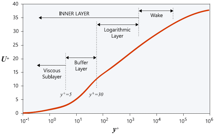
Fig. 11.3.1 Typical turbulent boundary-layer velocity profile and its near-wall regions.

Two approaches are generally used to model the near-wall region. In the first, the viscosity-affected inner region is not resolved. Semi-empirical wall functions bridge the viscous sublayer and buffer layer between the wall and the fully turbulent region. The high-Reynolds-number turbulence model then does not have to be modified to represent the wall itself.

In the second approach, usually called near-wall modeling or a wall-resolved treatment, the mesh extends through the viscosity-affected region to the wall. The turbulence model must then be modified so that it remains applicable within the viscous sublayer.

11.3.1. Standard Wall Functions

The standard \(k\)-\(\epsilon\) model is a high-Reynolds-number model. It is not directly applicable where viscous effects dominate close to a wall. Standard wall functions use an assumed universal form of the near-wall flow to bridge this region. This approach was introduced by Launder and Spalding for use with \(k\)-\(\epsilon\) models [LS74].

Near a wall, the wall-parallel mean velocity \(u\) depends principally on the normal distance \(y\), the density \(\rho\), the viscosity \(\mu\), and the wall shear stress \(\tau_w\). The friction velocity

(11.3.1.1)\[u_\tau=\sqrt{\frac{\tau_w}{\rho}}\]

provides the appropriate velocity scale. The nondimensional velocity and wall-normal distance are

(11.3.1.2)\[u^+=\frac{u}{u_\tau},\]

and

(11.3.1.3)\[y^+=\frac{\rho u_\tau y}{\mu}.\]

11.3.1.1. Linear Sublayer

The fluid is stationary at a no-slip wall, and turbulent eddy motion also vanishes very close to it. The viscous sublayer is generally thin, approximately \(y^+<5\), and its shear stress may be treated as constant and equal to the wall shear stress:

(11.3.1.4)\[\tau(y)=\mu\frac{du}{dy}=\tau_w.\]

Integration in the wall-normal direction gives

(11.3.1.5)\[u=\frac{\tau_wy}{\mu},\]

or, in wall coordinates,

(11.3.1.6)\[u^+=y^+.\]

11.3.1.2. Logarithmic Layer

Outside the viscous sublayer, a region exists in which turbulent transport is important and the shear stress varies slowly with distance from the wall. For a fully developed channel flow, assume that

1. convection is negligible,

2. the total shear stress is constant and equal to the wall shear stress, and

3. viscous shear is negligible relative to turbulent shear.

The Reynolds shear stress then satisfies

(11.3.1.7)\[-\widetilde{u''v''} \approx \frac{\tau_w}{\rho} = u_\tau^2.\]

Prandtl’s mixing-length model, with \(\ell_{\mathrm{mix}}=\kappa y\), gives

(11.3.1.8)\[\nu_t = (\kappa y)^2\left|\frac{du}{dy}\right|.\]

Combining the constant-shear approximation with the mixing-length relation gives

(11.3.1.9)\[u_\tau^2 = (\kappa y)^2 \left(\frac{du}{dy}\right)^2.\]

Integration produces the logarithmic law of the wall,

(11.3.1.10)\[u^+ = \frac{1}{\kappa}\ln y^+ + B = \frac{1}{\kappa}\ln(Ey^+),\]

where, for a smooth wall,

(11.3.1.11)\[E=9.793.\]

The logarithmic relation is typically associated with \(30<y^+<500\), although its actual range depends on the flow Reynolds number and pressure-gradient history.

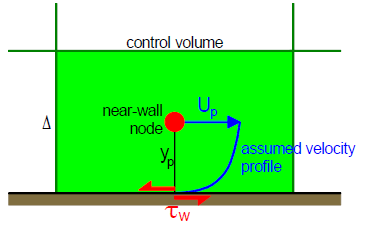
Fig. 11.3.1.1 Velocity profile in the near-wall region.

Using the eddy viscosity in Eq. (11.2.1.3) and assuming equilibrium between turbulence production and dissipation gives

(11.3.1.12)\[k=\frac{u_\tau^2}{\sqrt{C_\mu}}, \qquad \epsilon=\frac{u_\tau^3}{\kappa y}.\]

One possible wall-function procedure is to solve the logarithmic law iteratively for \(u_\tau\), using the wall-adjacent velocity \(u_P\) and distance \(y_P\), and then obtain \(\tau_w\). This procedure is acceptable in a nearly equilibrium boundary layer. Near separation or reattachment, however, \(u_P\) can vanish even while the turbulence remains substantial. The resulting \(u_\tau=0\) may have little immediate effect on the mean velocity, but it introduces errors in the \(k\) equation and can seriously degrade heat-transfer predictions.

When a transport equation is solved for \(k\), a more robust log-layer estimate uses the local turbulence kinetic energy:

(11.3.1.13)\[u_\tau=C_\mu^{1/4}k_P^{1/2}.\]

The value of \(\epsilon\) at the wall-adjacent point is then prescribed from the equilibrium relation. With the Boussinesq shear-stress approximation and the eddy-viscosity definition,

(11.3.1.14)\[\tau_w = \mu_t\frac{du}{dy} = C_\mu\rho\frac{k^2}{\epsilon}\frac{du}{dy}.\]

The standard wall function combines the linear and logarithmic laws:

(11.3.1.15)\[\begin{split}u^+ = \begin{cases} y^+, & y^+\le y_v^+,\\[2mm] \dfrac{1}{\kappa}\ln(Ey^+), & y^+>y_v^+. \end{cases}\end{split}\]

The transition coordinate \(y_v^+\) is the intersection of the two expressions. With Eq. (11.3.1.11), it is \(y_v^+=11.63\).

Stream implementation

The current \(k\)-\(\epsilon\) wall-function implementation uses \(\kappa=0.41\), \(E=9.0\), and a switching value of \(y_v^+=11.63\).

11.3.1.3. Momentum Equation

The strongest velocity gradients in a turbulent boundary layer occur near the wall. A wall-function calculation uses a comparatively coarse mesh, so the near-wall gradient is not resolved:

(11.3.1.16)\[\left.\mu\frac{\partial u}{\partial y}\right|_w \equiv \mu\frac{\Delta u}{\Delta y} > \mu\frac{u_P}{y_P}.\]

Here, \(P\) denotes the first interior solution point. In the inertial sublayer, the wall shear is therefore introduced as a source in the wall-adjacent momentum balance:

(11.3.1.17)\[S_w=\tau_w A,\]

where \(A\) is the area of the boundary face. The wall stress is estimated from

(11.3.1.18)\[\tau_w = \frac{ \rho C_\mu^{1/4}k_P^{1/2}u_P }{u^+}.\]

11.3.1.4. Treatment of \(k\) and \(\epsilon\) Near the Wall

Both \(k\) and \(\epsilon\) vary rapidly close to a wall. Because a standard wall-function mesh does not resolve those variations, the production and dissipation terms are modified and the value of \(\epsilon\) is specified directly rather than obtained from its transport equation.

For a simple two-dimensional boundary layer with \(y\) normal to the wall, the production term is

(11.3.1.19)\[P_k = - \rho\widetilde{u''v''}\frac{du}{dy} = \tau_w\frac{du}{dy}.\]

In the logarithmic region, production and dissipation are approximately in equilibrium:

(11.3.1.20)\[P_k=\rho\epsilon,\]

or

(11.3.1.21)\[\tau_w\frac{du}{dy}=\rho\epsilon.\]

The Boussinesq relation gives

(11.3.1.22)\[\tau_w = \mu_t\frac{du}{dy} = C_\mu\rho\frac{k^2}{\epsilon}\frac{du}{dy}.\]

The logarithmic wall law supplies

(11.3.1.23)\[\frac{du}{dy} = \frac{u_\tau}{\kappa y_P},\]

and the equilibrium dissipation is therefore

(11.3.1.24)\[\epsilon = \frac{u_\tau^3}{\kappa y_P}.\]

11.3.1.5. Energy Equation

Reynolds’ analogy between momentum and energy transport motivates a wall-temperature law with two profile assumptions:

• a linear profile in the thermal conduction sublayer, where molecular conduction is important; and

• a logarithmic profile in the turbulent region, where turbulent transport dominates conduction.

The thermal conduction layer need not have the same thickness as the momentum viscous sublayer. Their approximate relation depends on the molecular Prandtl number:

(11.3.1.25)\[\frac{\delta}{\delta_T}\approx\sqrt{Pr}.\]

The normalized temperature is

(11.3.1.26)\[T^+ \equiv - \frac{(T_P-T_w)C_p\mu u_\tau}{q_w} = \sigma_t \left[ u^+ + P\left(\frac{\sigma_l}{\sigma_t}\right) \right],\]

where \(T_P\) is the wall-adjacent temperature, \(T_w\) is the wall temperature, \(C_p\) is the specific heat at constant pressure, \(q_w\) is the wall heat flux, \(\sigma_t\) is the turbulent Prandtl number, \(\sigma_l=\mu C_p/\Gamma_T\) is the molecular Prandtl number, and \(\Gamma_T\) is the thermal conductivity.

The function \(P\) corrects for the ratio of molecular to turbulent Prandtl numbers. Jayatilleke’s expression is [Jay69]

(11.3.1.27)\[P\left(\frac{\sigma_l}{\sigma_t}\right) = 9.24 \left[ \left(\frac{\sigma_l}{\sigma_t}\right)^{0.75} -1 \right] \left\{ 1+0.28 \exp\left[ -0.007\left(\frac{\sigma_l}{\sigma_t}\right) \right] \right\}.\]

The standard wall-function procedure can now be summarized without removing the intermediate physics developed above:

1. Compute the friction velocity:

   (11.3.1.28)\[u_\tau=C_\mu^{1/4}k_P^{1/2}.\]

2. Compute the wall coordinate:

   (11.3.1.29)\[y^+=\frac{\rho u_\tau y_P}{\mu},\]

   and evaluate \(u^+\) from Eq. (11.3.1.15).

3. Apply the wall shear to the momentum equation:

   (11.3.1.30)\[\tau_w=\frac{\rho u_\tau u_P}{u^+}, \qquad \boldsymbol{F}_w=-\boldsymbol{\tau}_wA.\]

   This form covers both the linear sublayer and the logarithmic layer.

4. Evaluate production and destruction in the \(k\) equation:

   (11.3.1.31)\[P_{k,P} = \tau_w\frac{u_P}{y_P}, \qquad \rho\epsilon_P = \frac{ \rho C_\mu^{3/4}k_P^{3/2} }{\kappa y_P}.\]

5. Do not solve the wall-adjacent \(\epsilon\) equation; prescribe

   (11.3.1.32)\[\epsilon_P = \frac{ C_\mu^{3/4}k_P^{3/2} }{\kappa y_P}.\]

6. Apply the wall heat flux to the energy equation:

   (11.3.1.33)\[q_w = - \frac{ \rho C_pC_\mu^{1/4}k_P^{1/2}(T_P-T_w) }{T^+}.\]

The useful \(y^+\) range of a wall function depends on the Reynolds number of the flow. The lower limit is generally of order 15; below it, the accuracy of a standard logarithmic wall function deteriorates. The upper limit depends strongly on Reynolds number. The logarithmic layer can extend to several thousand wall units for high-Reynolds-number ship or aircraft flows, whereas its upper limit can be near 100 in a lower-Reynolds-number turbine-blade flow. In such lower-Reynolds-number flows, the entire boundary layer may span only a few hundred wall units, and imposing a wall-function placement can prevent the use of enough cells through the boundary layer. Adequate resolution across the complete boundary layer remains more important than targeting one isolated \(y^+\) value.

11.4. Two-Layer \(k\)-\(\epsilon\) Model

The enhanced \(k\)-\(\epsilon\) treatment combines a two-layer zonal model with a blended law of the wall. The two-layer model modifies the treatment of the \(\epsilon\) equation and the eddy viscosity in the near-wall region and uses a blending function to join that region to the outer flow.

If the near-wall mesh resolves the viscous sublayer, with its first solution point at approximately \(y^+=1\), the treatment reverts to the traditional two-layer zonal model of Chen and Patel [CP88]. Requiring every wall region in a complex grid to have that resolution may be too expensive, however. The enhanced model is therefore designed for coarse wall-function meshes as well as fine low-Reynolds-number meshes. It also provides a continuous treatment when an intermediate mesh places the first point in the buffer region, where neither a fully turbulent wall function nor direct viscous-sublayer resolution is ideal. Its objective is to retain the accuracy of the traditional two-layer approach in wall-resolved regions while providing a reasonable wall-function treatment in coarser regions.

The model divides the flow into two zones on a cell-by-cell basis. The wall-distance Reynolds number is

(11.4.1)\[Re_y = \frac{\rho y\sqrt{k}}{\mu},\]

where \(y\) is the distance from the cell center to the nearest wall. The zones are

(11.4.2)\[\begin{split}\begin{aligned} Re_y&<Re_y^*, &&\text{viscosity-affected region},\\ Re_y&>Re_y^*, &&\text{fully turbulent region}, \end{aligned} \qquad Re_y^*=200\end{split}\]

in the original formulation.

In the fully turbulent region, the standard \(k\)-\(\epsilon\) model is used and the momentum, \(k\), and \(\epsilon\) equations are solved. In the viscosity-affected region, the one-equation model of Wolfshtein [Wol69] is used. The momentum and \(k\) equations are retained, but the viscous-region dissipation is computed algebraically:

(11.4.3)\[\epsilon_{\mathrm{vis}} = \frac{k^{3/2}}{\ell_\epsilon}.\]

The Chen–Patel length scale is

(11.4.4)\[\ell_\epsilon = C_\ell y \left[ 1- \exp\left(-\frac{Re_y}{A_\epsilon}\right) \right].\]

The effective dissipation is obtained by blending the transport-equation value with the algebraic near-wall value:

(11.4.5)\[\epsilon_{\mathrm{eff}} = \lambda_\epsilon\epsilon_{\mathrm{transport}} + \left(1-\lambda_\epsilon\right) \epsilon_{\mathrm{vis}}.\]

The blending function varies smoothly from zero near a wall to one in the outer region:

(11.4.6)\[\lambda_\epsilon = \frac{1}{2} \left[ 1+ \tanh\left( \frac{Re_y-Re_y^*}{A} \right) \right].\]

If the transition width \(\Delta Re_y\) is defined so that \(\lambda_\epsilon\) lies within one percent of its far-field value, then

(11.4.7)\[A = \frac{\Delta Re_y}{\operatorname{atanh}(0.98)}.\]

A typical choice for \(\Delta Re_y\) is between 5% and 20% of \(Re_y^*\). The smooth transition prevents convergence from being impeded when \(\epsilon_{\mathrm{transport}}\) does not exactly match \(\epsilon_{\mathrm{vis}}\) at the edge of the viscosity-affected region.

The eddy viscosity in that region is also evaluated algebraically:

(11.4.8)\[\mu_{t,\mathrm{vis}} = \rho C_\mu\ell_\mu\sqrt{k},\]

with

(11.4.9)\[\ell_\mu = C_\ell y \left[ 1- \exp\left(-\frac{Re_y}{A_\mu}\right) \right].\]

Its effective value is

(11.4.10)\[\mu_{t,\mathrm{eff}} = \lambda_\epsilon\mu_t + \left(1-\lambda_\epsilon\right) \mu_{t,\mathrm{vis}}.\]

The Chen–Patel constants are

(11.4.11)\[C_\ell = \kappa C_\mu^{-3/4}, \qquad A_\epsilon=2C_\ell, \qquad A_\mu=70.\]

The blending of both \(\epsilon\) and \(\mu_t\) provides a smooth transition between their transported outer-region values and their algebraic viscosity-affected values.

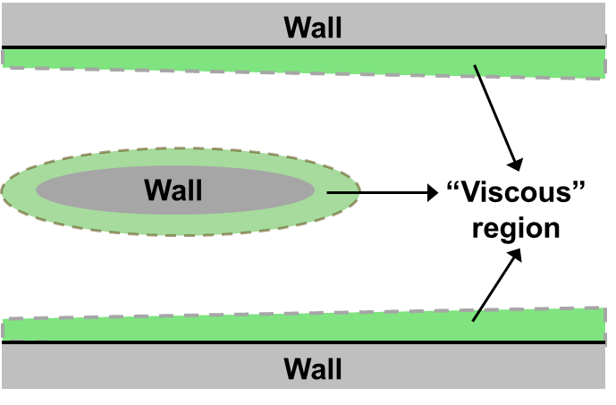
Fig. 11.4.1 The viscosity-affected and fully turbulent regions in the two-layer \(k\)-\(\epsilon\) model.

Stream implementation

The original formulation above uses \(Re_y^*=200\) as its nominal division. The current Stream implementation defaults to \(Re_y^*=75\) and \(\Delta Re_y=0.15Re_y^*\). It also forces the outer branch when \(y^+>200\), preventing a small value of \(k\) far from a wall from spuriously selecting the inner model. These are implementation choices rather than universal constants of the two-layer model.

11.4.1. Enhanced Wall Functions

The enhanced wall functions allow the same treatment to be used throughout the viscosity-affected region, regardless of whether a wall-adjacent point lies in the viscous sublayer, buffer region, or fully turbulent region. They differ from the standard wall functions in two principal ways:

1. they blend the linear laminar velocity profile with the logarithmic turbulent law of the wall; and

2. they extend the wall law to account for pressure gradient, wall heat transfer, and compressibility.

The linear and logarithmic velocity profiles are blended using

(11.4.1.1)\[u^+ = e^\Gamma u_{\mathrm{lam}}^+ + e^{1/\Gamma}u_{\mathrm{turb}}^+,\]

where the Kader-type blending function is [Kad81]

(11.4.1.2)\[\Gamma = - \frac{a(y^+)^4}{1+by^+}, \qquad a=0.01, \qquad b=5.\]

The derivative is blended in the corresponding form:

(11.4.1.3)\[\frac{du^+}{dy^+} = e^\Gamma \frac{du_{\mathrm{lam}}^+}{dy^+} + e^{1/\Gamma} \frac{du_{\mathrm{turb}}^+}{dy^+}.\]

This construction recovers the appropriate asymptotic behavior for both small and large \(y^+\) while retaining a smooth representation through the buffer region.

White and Christoph extended the wall law to compressible flow with pressure gradient and heat transfer [WC72]. The near-wall velocity profile is expressed in terms of the inner coordinates and three parameters:

(11.4.1.4)\[u^+ = f\left( y^+, \text{pressure gradient}, \text{heat transfer}, \text{compressibility} \right) = f(y^+,\alpha,\beta,\gamma).\]

The pressure-gradient, heat-transfer, and compressibility parameters are

(11.4.1.5)\[\alpha \equiv \frac{\nu_w}{\tau_wu_\tau}\frac{dp}{dx} = \frac{\mu}{\rho^2u_\tau^3}\frac{dp}{dx},\]

(11.4.1.6)\[\beta \equiv \frac{Pr_tq_wu_\tau}{C_p\tau_wT_w} = \frac{Pr_tq_w}{\rho C_pu_\tau T_w},\]

and

(11.4.1.7)\[\gamma \equiv \frac{Pr_tu_\tau^2}{2C_pT_w}.\]

The turbulent part of the extended wall law satisfies

(11.4.1.8)\[\frac{du_{\mathrm{turb}}^+}{dy^+} = \frac{1}{\kappa y^+} S^{1/2} \left[ 1+\beta u^+-\gamma(u^+)^2 \right]^{1/2}.\]

With an initial condition \((u_0^+,y_0^+)\), integration gives

(11.4.1.9)\[u_{\mathrm{turb}}^+ = \frac{1}{2\gamma} \left[ \beta + Q\sin \left\{ \phi + \frac{\sqrt{\gamma}}{\kappa} \left[ 2(S-S_0) + \ln\left( \frac{S-1}{S+1} \frac{S_0+1}{S_0-1} \right) \right] \right\} \right],\]

where

(11.4.1.10)\[\phi = \sin^{-1} \left( \frac{2\gamma u_0^+-\beta}{Q} \right), \qquad Q=\sqrt{\beta^2+4\gamma}, \qquad S=\sqrt{1+\alpha y^+}.\]

In the zero-pressure-gradient, adiabatic, incompressible limit, this expression reduces to the standard logarithmic law,

(11.4.1.11)\[u^+(y^+,0,0,0) = \frac{1}{\kappa}\ln y^+ + B.\]

The no-slip point supplies the initial condition

(11.4.1.12)\[u_0^+=0 \quad\text{at}\quad y_0^+=e^{-\kappa B} = 0.1108 \quad \text{for }\kappa=0.4\text{ and }B=5.5.\]

11.5. Buoyancy Correction in the \(k\)-\(\epsilon\) Models

When a temperature gradient and a nonzero gravity field occur together, buoyancy can generate or suppress turbulence kinetic energy. A source is therefore added to the \(k\) equation, with a corresponding possible source in the \(\epsilon\) equation. The buoyancy production is

(11.5.1)\[P_b = \beta g_i \frac{\mu_t}{Pr_t} \frac{\partial T}{\partial x_i},\]

where \(Pr_t\) is the turbulent Prandtl number for energy and \(g_i\) is the \(i\)-direction component of gravity. Its default value for the \(k\)-\(\epsilon\) models is 0.85. The thermal-expansion coefficient is

(11.5.2)\[\beta = - \frac{1}{\rho} \left( \frac{\partial\rho}{\partial T} \right)_p.\]

For an ideal gas, the production may be written

(11.5.3)\[P_b = - g_i \frac{\mu_t}{\rho Pr_t} \frac{\partial\rho}{\partial x_i}.\]

Unstable stratification gives \(P_b>0\) and augments turbulence kinetic energy; stable stratification gives \(P_b<0\) and suppresses it. The buoyancy contribution to the \(k\) equation is comparatively well established and is normally included when gravity and temperature or density gradients are present together. Its effect on \(\epsilon\) is less certain, so the corresponding \(\epsilon\)-equation source is commonly omitted by default.

When that source is included, \(C_{3\epsilon}\) in Eq. (11.2.1.2) is estimated as

(11.5.4)\[C_{3\epsilon} = \tanh\left| \frac{v}{u} \right|,\]

where \(v\) is the velocity component parallel to gravity and \(u\) is the component perpendicular to gravity. Thus, \(C_{3\epsilon}\) approaches one when the principal direction of a buoyant shear layer is aligned with gravity and approaches zero when it is perpendicular to gravity.

11.6. \(k\)-\(\omega\) Model

The \(k\)-\(\omega\) model solves transport equations for turbulence kinetic energy \(k\) and its specific dissipation rate \(\omega\). The latter may be interpreted as being proportional to \(\epsilon/k\). The modeled equations are

(11.6.1)\[\frac{\partial(\rho k)}{\partial t} + \frac{\partial(\rho u_i k)}{\partial x_i} = \frac{\partial}{\partial x_i} \left[ \left(\mu+\sigma_k\mu_t\right) \frac{\partial k}{\partial x_i} \right] + P_k-Y_k,\]

and

(11.6.2)\[\frac{\partial(\rho\omega)}{\partial t} + \frac{\partial(\rho u_i\omega)}{\partial x_i} = \frac{\partial}{\partial x_i} \left[ \left(\mu+\sigma_\omega\mu_t\right) \frac{\partial\omega}{\partial x_i} \right] + P_\omega-Y_\omega.\]

The turbulent viscosity is

(11.6.3)\[\mu_t = \alpha^*\frac{\rho k}{\omega}.\]

The production of \(k\) is

(11.6.4)\[P_k = - \rho\widetilde{u_i''u_j''} \frac{\partial u_j}{\partial x_i},\]

which, under the Boussinesq hypothesis, is written as

(11.6.5)\[P_k=\mu_tS^2.\]

The production of \(\omega\) is modeled as

(11.6.6)\[P_\omega = \gamma^*\frac{\omega}{k}P_k = \gamma^*\alpha^*\frac{\rho}{\mu_t}P_k.\]

The dissipation of \(k\) is

(11.6.7)\[Y_k = \rho\beta^*f_{\beta^*}k\omega,\]

where

(11.6.8)\[\begin{split}f_{\beta^*} = \begin{cases} 1, &\chi_k\le0,\\[2mm] \dfrac{1+680\chi_k^2}{1+400\chi_k^2}, &\chi_k>0, \end{cases}\end{split}\]

with

(11.6.9)\[\chi_k^2 = \frac{1}{\omega^3} \frac{\partial k}{\partial x_j} \frac{\partial\omega}{\partial x_j}.\]

The compressibility-dependent coefficient is

(11.6.10)\[\beta^* = \beta_i^* \left[ 1+\zeta^*F(M_t) \right],\]

where, in the high-Reynolds-number form,

(11.6.11)\[\beta_i^*=\beta_\infty^*.\]

The dissipation of \(\omega\) is

(11.6.12)\[Y_\omega = \rho\beta f_\beta\omega^2,\]

with

(11.6.13)\[f_\beta = \frac{1+70\chi_\omega}{1+80\chi_\omega},\]

(11.6.14)\[\chi_\omega = \left| \frac{\Omega_{ij}\Omega_{jk}S_{ki}} {\left(\beta_\infty^*\omega\right)^3} \right|,\]

and

(11.6.15)\[\Omega_{ij} = \frac{1}{2} \left( \frac{\partial u_i}{\partial x_j} - \frac{\partial u_j}{\partial x_i} \right).\]

The coefficient \(\beta\) is

(11.6.16)\[\beta = \beta_i \left[ 1- \frac{\beta_i^*}{\beta_i} \zeta^*F(M_t) \right].\]

11.6.1. Compressibility Correction

The compressibility function in Eqs. (11.6.10) and (11.6.16) is

(11.6.1.1)\[\begin{split}F(M_t) = \begin{cases} 0, &M_t\le M_{t0},\\ M_t^2-M_{t0}^2, &M_t>M_{t0}, \end{cases}\end{split}\]

where the turbulent Mach number and ideal-gas speed of sound are

(11.6.1.2)\[M_t^2=\frac{2k}{a^2}, \qquad a=\sqrt{\gamma RT}.\]

11.6.2. \(k\)-\(\omega\) Model Constants

The model constants are

(11.6.2.1)\[\alpha^*=1, \qquad \alpha_0^*=0.024, \qquad \gamma^*=0.52, \qquad \gamma_0=\frac{1}{9}, \qquad \beta_i^*=0.09, \qquad \beta_i=0.072, \qquad R_\beta=8,\]

and

(11.6.2.2)\[R_k=6, \qquad R_\omega=2.95, \qquad \zeta^*=1.5, \qquad M_{t0}=0.25, \qquad \sigma_k=0.5, \qquad \sigma_\omega=0.5.\]

Model context

This standard \(k\)-\(\omega\) formulation supplies the theoretical foundation for the Menter baseline and SST models that follow. The current Stream turbulence-model selector exposes the Menter families rather than a separate standalone standard \(k\)-\(\omega\) option.

11.7. Menter Baseline and Shear-Stress-Transport Models

Menter’s baseline (BSL) and shear-stress-transport (SST) models are closely related. Their principal differences are the eddy-viscosity definition and some model constants. Their governing equations are

(11.7.1)\[\frac{\partial(\rho k)}{\partial t} + \frac{\partial(\rho u_i k)}{\partial x_i} = \frac{\partial}{\partial x_i} \left[ \left(\mu+\sigma_k\mu_t\right) \frac{\partial k}{\partial x_i} \right] + P_k-Y_k,\]

and

(11.7.2)\[\frac{\partial(\rho\omega)}{\partial t} + \frac{\partial(\rho u_i\omega)}{\partial x_i} = \frac{\partial}{\partial x_i} \left[ \left(\mu+\sigma_\omega\mu_t\right) \frac{\partial\omega}{\partial x_i} \right] + P_\omega-Y_\omega+D_\omega.\]

The eddy viscosity is

(11.7.3)\[\begin{split}\mu_t = \begin{cases} \alpha^*\dfrac{\rho k}{\omega}, &\text{BSL},\\[4mm] \dfrac{\rho k}{\omega} \dfrac{1}{ \max\left( \dfrac{1}{\alpha^*}, \dfrac{\Omega F_2}{a_1\omega} \right) }, &\text{SST}. \end{cases}\end{split}\]

The diffusion coefficients blend inner and outer values:

(11.7.4)\[\sigma_k = F_1\sigma_{k1} + (1-F_1)\sigma_{k2},\]

(11.7.5)\[\sigma_\omega = F_1\sigma_{\omega1} + (1-F_1)\sigma_{\omega2}.\]

The vorticity magnitude is

(11.7.6)\[\Omega = \sqrt{2\Omega_{ij}\Omega_{ij}}.\]

The first blending function is

(11.7.7)\[F_1=\tanh\left(\Gamma_1^4\right),\]

with

(11.7.8)\[\Gamma_1 = \min \left[ \max \left( \frac{\sqrt{k}}{0.09\,\omega d}, \frac{500\mu}{\rho d^2\omega} \right), \frac{4\rho k\sigma_{\omega2}}{D_\omega^+d^2} \right],\]

and

(11.7.9)\[D_\omega^+ = \max \left[ \frac{2\sigma_{\omega2}\rho}{\omega} \frac{\partial k}{\partial x_j} \frac{\partial\omega}{\partial x_j}, 10^{-20} \right].\]

The second blending function is

(11.7.10)\[F_2=\tanh\left(\Gamma_2^2\right),\]

where

(11.7.11)\[\Gamma_2 = \max \left[ \frac{2\sqrt{k}}{0.09\,\omega d}, \frac{500\mu}{\rho d^2\omega} \right].\]

Here, \(d\) is the normal distance to the nearest wall and \(D_\omega^+\) is the positive part of the cross-diffusion term.

The \(k\)-production term is the same as in the standard \(k\)-\(\omega\) model, whereas production of \(\omega\) is

(11.7.12)\[P_\omega = \gamma^*\frac{\rho}{\mu_t}P_k.\]

This differs from the corresponding standard-model expression. The coefficient is blended:

(11.7.13)\[\gamma^* = F_1\gamma_1+(1-F_1)\gamma_2,\]

where

(11.7.14)\[\gamma_1 = \frac{\beta_{i1}}{\beta_i^*} - \frac{\kappa^2\sigma_{\omega1}}{\sqrt{\beta_i^*}} = 0.55,\]

and

(11.7.15)\[\gamma_2 = \frac{\beta_{i2}}{\beta_i^*} - \frac{\kappa^2\sigma_{\omega2}}{\sqrt{\beta_i^*}} = 0.44.\]

Here, \(\kappa=0.41\), \(\beta_{i1}=0.075\), and \(\beta_{i2}=0.0828\).

The dissipation terms retain the standard \(k\)-\(\omega\) form but set both correction functions to unity:

(11.7.16)\[Y_k=\rho\beta^*k\omega, \qquad Y_\omega=\rho\beta\omega^2.\]

The coefficient \(\beta_i\) is blended as

(11.7.17)\[\beta_i = F_1\beta_{i1} + (1-F_1)\beta_{i2},\]

where

(11.7.18)\[\beta_{i1}=0.075, \qquad \beta_{i2}=0.0828.\]

The cross-diffusion term arises from transforming an \(\epsilon\) equation into an \(\omega\) equation:

(11.7.19)\[D_\omega = 2(1-F_1) \frac{\rho\sigma_{\omega2}}{\omega} \frac{\partial k}{\partial x_j} \frac{\partial\omega}{\partial x_j}.\]

The remaining model constants are

(11.7.20)\[\sigma_{\omega1}=0.5, \qquad \sigma_{k2}=1.0, \qquad \sigma_{\omega2}=0.856, \qquad \beta_{i1}=0.075, \qquad \beta_{i2}=0.0828,\]

with

(11.7.21)\[\begin{split}\sigma_{k1} = \begin{cases} 0.5,&\text{BSL},\\ 0.85,&\text{SST}, \end{cases}\end{split}\]

and, for SST only,

(11.7.22)\[a_1=0.31.\]

All other constants retain their standard \(k\)-\(\omega\) values.

11.8. Original SST and SST-2003

The original SST model of Menter [Men94] and the modified SST-2003 model [MKL03, Rum03] can be compared directly by writing their governing equations as

(11.8.1)\[\frac{\partial(\rho k)}{\partial t} + \frac{\partial(\rho u_i k)}{\partial x_i} = \frac{\partial}{\partial x_i} \left[ \left(\mu+\sigma_k\mu_t\right) \frac{\partial k}{\partial x_i} \right] + \widetilde{P}_k - \beta^*\rho k\omega,\]

and

(11.8.2)\[\begin{split}\begin{aligned} \frac{\partial(\rho\omega)}{\partial t} + \frac{\partial(\rho u_i\omega)}{\partial x_i} ={}& \frac{\partial}{\partial x_i} \left[ \left(\mu+\sigma_\omega\mu_t\right) \frac{\partial\omega}{\partial x_i} \right] + \gamma\frac{\rho}{\mu_t}\widetilde{P}_k - \beta\rho\omega^2 \\ &+ 2(1-F_1) \rho\sigma_{\omega2} \frac{1}{\omega} \frac{\partial k}{\partial x_j} \frac{\partial\omega}{\partial x_j}. \end{aligned}\end{split}\]

The final term in the \(\omega\) equation is the cross-diffusion term created by transforming the outer \(k\)-\(\epsilon\) model to an \(\omega\)-equation form.

The first difference between the two SST versions is the turbulent-viscosity limiter:

(11.8.3)\[\begin{split}\mu_t = \begin{cases} \dfrac{\rho k}{\omega} \dfrac{1}{ \max\left( 1,\dfrac{\Omega F_2}{a_1\omega} \right) }, &\text{original SST},\\[5mm] \dfrac{\rho k}{\omega} \dfrac{1}{ \max\left( 1,\dfrac{SF_2}{a_1\omega} \right) }, &\text{SST-2003}. \end{cases}\end{split}\]

Equivalently,

(11.8.4)\[\begin{split}\mu_t = \begin{cases} \dfrac{a_1\rho k} {\max(a_1\omega,\Omega F_2)}, &\text{original SST},\\[4mm] \dfrac{a_1\rho k} {\max(a_1\omega,SF_2)}, &\text{SST-2003}. \end{cases}\end{split}\]

The original model limits the eddy viscosity using the vorticity magnitude, whereas SST-2003 uses the strain-rate magnitude.

The unmodified production term is

(11.8.5)\[P_k = \tau_{ij}\frac{\partial u_j}{\partial x_i},\]

with the Boussinesq stress

(11.8.6)\[\tau_{ij} = \mu_t \left( 2S_{ij} - \frac{2}{3} \frac{\partial u_k}{\partial x_k} \delta_{ij} \right) - \frac{2}{3}\rho k\delta_{ij},\]

and

(11.8.7)\[S_{ij} = \frac{1}{2} \left( \frac{\partial u_i}{\partial x_j} + \frac{\partial u_j}{\partial x_i} \right).\]

SST-2003 limits production to avoid excessive turbulence buildup in stagnation regions:

(11.8.8)\[\begin{split}\widetilde{P}_k = \begin{cases} P_k, &\text{original SST},\\[1mm] \min\left( P_k, 10\beta^*\rho k\omega \right), &\text{SST-2003}. \end{cases}\end{split}\]

The strain-rate and rotation-rate magnitudes used above are

(11.8.9)\[S=\sqrt{2S_{ij}S_{ij}},\]

and

(11.8.10)\[\Omega_{ij} = \frac{1}{2} \left( \frac{\partial u_i}{\partial x_j} - \frac{\partial u_j}{\partial x_i} \right), \qquad \Omega=\sqrt{2\Omega_{ij}\Omega_{ij}}.\]

The blending functions retain the forms

(11.8.11)\[F_1=\tanh\left(\Gamma_1^4\right),\]

(11.8.12)\[\Gamma_1 = \min \left[ \max \left( \frac{\sqrt{k}}{0.09\,\omega d}, \frac{500\mu}{\rho\omega d^2} \right), \frac{4\rho\sigma_{\omega2}k} {CD_{k\omega}d^2} \right],\]

where

(11.8.13)\[\begin{split}CD_{k\omega} = \begin{cases} \displaystyle \max\left[ \frac{2\rho\sigma_{\omega2}}{\omega} \frac{\partial k}{\partial x_j} \frac{\partial\omega}{\partial x_j}, 10^{-20} \right], &\text{original SST},\\[5mm] \displaystyle \max\left[ \frac{2\rho\sigma_{\omega2}}{\omega} \frac{\partial k}{\partial x_j} \frac{\partial\omega}{\partial x_j}, 10^{-10} \right], &\text{SST-2003}, \end{cases}\end{split}\]

and

(11.8.14)\[F_2=\tanh\left(\Gamma_2^2\right), \qquad \Gamma_2 = \max \left[ \frac{2\sqrt{k}}{0.09\,\omega d}, \frac{500\mu}{\rho\omega d^2} \right].\]

The constants \(\sigma_k\), \(\sigma_\omega\), \(\gamma\), and \(\beta\) are blended between their near-wall and outer values:

(11.8.15)\[\begin{split}\begin{aligned} \sigma_k &= F_1\sigma_{k1} + (1-F_1)\sigma_{k2}, \\ \sigma_\omega &= F_1\sigma_{\omega1} + (1-F_1)\sigma_{\omega2}, \\ \gamma &= F_1\gamma_1 + (1-F_1)\gamma_2, \\ \beta &= F_1\beta_1 + (1-F_1)\beta_2. \end{aligned}\end{split}\]

Their component values are

(11.8.16)\[\sigma_{k1}=0.85, \qquad \sigma_{k2}=1.0, \qquad \sigma_{\omega1}=0.5, \qquad \sigma_{\omega2}=0.856,\]

(11.8.17)\[\gamma_1=\frac{5}{9}, \qquad \gamma_2=0.44, \qquad \beta_1=0.075, \qquad \beta_2=0.0828.\]

The remaining constants are

(11.8.18)\[a_1=0.31, \qquad \beta^*=0.09.\]

Stream implementation

In the current Stream implementation, the BSL and original-SST families use an upper production limit of \(20\beta^*\rho k\omega\). SST-2003 uses the \(10\beta^*\rho k\omega\) limit shown above and applies the limited production consistently to both transport equations.

11.9. Near-Wall Turbulence Treatment for SST Models

Turbulent-flow simulations are difficult near solid walls because the mean velocity and, for nonadiabatic walls, temperature gradients become steep. Directly resolving those gradients requires a boundary-layer grid that is fine in at least the wall-normal direction and therefore increases computational cost. More fundamentally, the wall damps turbulent fluctuations and lowers the local turbulence Reynolds number, so the turbulence closure must respond to the local near-wall structure. In an SST model, empirical blending and eddy-viscosity limiting provide this low-Reynolds-number response through the wall distance and the local strain-rate or vorticity magnitude.

Two treatments are possible. In a low-Reynolds-number treatment, the SST model is integrated directly through the boundary layer to the wall. In a law-of-the-wall treatment, empirical algebraic profiles relate the velocity and temperature at the first cell away from the wall to the wall shear and heat flux, avoiding the requirement to resolve the complete near-wall profile. The unified law presented here covers the viscous sublayer, buffer layer, and logarithmic layer up to approximately \(y^+=100\).

The wall-parallel velocity profile is written as

(11.9.1)\[y^+ = u^+ + y_{\mathrm{white}}^+ - e^{-\kappa B} \left[ 1+\kappa u^+ + \frac{(\kappa u^+)^2}{2} + \frac{(\kappa u^+)^3}{6} \right],\]

where

(11.9.2)\[y_{\mathrm{white}}^+ = \exp \left[ \frac{\kappa}{\sqrt{\Gamma}} \left\{ \sin^{-1} \left( \frac{2\Gamma u^+-\beta}{Q} \right) - \Phi \right\} \right] \exp(-\kappa B).\]

The inner variables and wall-law parameters are

(11.9.3)\[u^+=\frac{u}{u_\tau}, \qquad y^+=\frac{u_\tau y}{\nu}, \qquad u_\tau=\sqrt{\frac{\tau_w}{\rho}},\]

(11.9.4)\[\kappa=0.41, \qquad B=5.5, \qquad \Gamma = \frac{Pr^{1/3}u_\tau^2}{2C_pT_w}, \qquad \beta = \frac{q_w\nu_w}{T_wK_wu_\tau},\]

and

(11.9.5)\[\Phi = \sin^{-1}\left(-\frac{\beta}{Q}\right), \qquad Q=\sqrt{\beta^2+4\Gamma}, \qquad y_0^+=e^{-\kappa B}.\]

Here, \(K_w\) and \(\nu_w\) are the wall thermal conductivity and kinematic viscosity. Once \(u^+\) has been obtained, the near-wall temperature is

(11.9.6)\[T = T_w \left[ 1+\beta u^+-\Gamma(u^+)^2 \right].\]

11.10. Variants of the BSL and SST Models

The BSL and SST production terms can be modified in several useful ways. In the first modification, the isotropic \(\tfrac{2}{3}\rho k\delta_{ij}\) contribution in the Boussinesq stress is ignored in the momentum and energy equations, and production is approximated as

(11.10.1)\[P_k=\mu_tS^2.\]

This expression is exact for incompressible flow and is normally a good approximation except, potentially, at very high Mach number. The corresponding models are denoted BSL-m and SST-m.

A second set of variants uses the vorticity magnitude

(11.10.2)\[\Omega=\sqrt{2\Omega_{ij}\Omega_{ij}}.\]

The vorticity-based source is often close to the exact source in a simple boundary layer, is readily available, and can avoid numerical difficulties associated with the exact production term. The BSL-V and SST-V variants use

(11.10.3)\[P_k = \mu_t\Omega^2 - \frac{2}{3}\rho k(\boldsymbol{\nabla}\cdot\boldsymbol{u}).\]

If the isotropic \(k\) term is also omitted, the BSL-Vm and SST-Vm variants use

(11.10.4)\[P_k=\mu_t\Omega^2.\]

The Kato–Launder correction uses \(\mu_tS\Omega\) in place of \(\mu_t\Omega^2\) [KL93]. The BSL-KL and SST-KL variants retain the isotropic contribution:

(11.10.5)\[P_k = \mu_tS\Omega - \frac{2}{3}\rho k(\boldsymbol{\nabla}\cdot\boldsymbol{u}),\]

whereas BSL-KLm and SST-KLm omit it:

(11.10.6)\[P_k=\mu_tS\Omega.\]

The same modifications apply to SST-2003. For reference, the unsuffixed compressible production form is

(11.10.7)\[P_k = \mu_t \left[ S^2 - \frac{2}{3} \left( \boldsymbol{\nabla}\cdot\boldsymbol{u} \right)^2 \right] - \frac{2}{3} \rho k \left( \boldsymbol{\nabla}\cdot\boldsymbol{u} \right).\]

The production choices and their original motivations are summarized below.

Model variant	Production before model limiting	Principal motivation
BSL-m, SST-m	\(\mu_tS^2\)	Good approximation except, potentially, at very high Mach number
BSL-V, SST-V	\(\mu_t\Omega^2-\tfrac{2}{3}\rho k\nabla\cdot\boldsymbol{u}\)	Replaces the exact source by a vorticity source that behaves similarly in simple boundary layers
BSL-Vm, SST-Vm	\(\mu_t\Omega^2\)	Often favored for hypersonic flows, particularly in the presence of strong shocks
BSL-KL, SST-KL	\(\mu_tS\Omega-\tfrac{2}{3}\rho k\nabla\cdot\boldsymbol{u}\)	Kato–Launder correction, similar in intent to the vorticity variant
BSL-KLm, SST-KLm	\(\mu_tS\Omega\)	Kato–Launder correction with the isotropic \(k\) term omitted
SST-2003	Eq. (11.10.7)	Uses the SST-2003 production limiter
SST-2003-m	\(\mu_tS^2\)	Modified strain production with the SST-2003 limiter
SST-2003-V	\(\mu_t\Omega^2-\tfrac{2}{3}\rho k\nabla\cdot\boldsymbol{u}\)	Vorticity production with the SST-2003 limiter
SST-2003-Vm	\(\mu_t\Omega^2\)	Modified vorticity production with the SST-2003 limiter
SST-2003-KL	\(\mu_tS\Omega-\tfrac{2}{3}\rho k\nabla\cdot\boldsymbol{u}\)	Kato–Launder production with the SST-2003 limiter
SST-2003-KLm	\(\mu_tS\Omega\)	Modified Kato–Launder production with the SST-2003 limiter

The suffix changes the production definition. It does not change the blending functions, eddy-viscosity definition, or constants of the selected BSL, SST, or SST-2003 family.

Stream model names

The corresponding current selectors are menterBSL, menterSST, and menterSST2003, followed where appropriate by _m, _V, _Vm, _KL, or _KLm. The current BSL and original-SST variants use the family production limit \(20\beta^*\rho k\omega\); the SST-2003 variants use \(10\beta^*\rho k\omega\).

For compressible flow, the implementation retains the deviatoric-strain correction \(-\tfrac{2}{3}\mu_t(\boldsymbol{\nabla}\cdot\boldsymbol{u})^2\) in every production variant. The m suffix removes only the isotropic \(-\tfrac{2}{3}\rho k(\boldsymbol{\nabla}\cdot\boldsymbol{u})\) contribution. Consequently, the compact production expressions in the table above are recovered exactly for incompressible flow; their current compressible forms also contain the deviatoric-strain correction.

11.11. Specification of \(k\) and \(\omega\) at Inlets

The inlet values of \(k\) and \(\omega\) should produce a physically reasonable ratio of eddy viscosity to molecular viscosity. Because the high-Reynolds-number eddy viscosity is approximately \(\rho k/\omega\), specifying \(k\) too low or \(\omega\) too high can make this ratio unreasonably small. Recommendations in Menter’s original SST paper were developed for external aerodynamic flows and can produce eddy viscosities below the molecular viscosity; they should not be transferred directly to internal flows.

11.11.1. Turbulence Intensity

Turbulence intensity is the ratio of the root-mean-square velocity fluctuation to a representative mean free-stream velocity:

(11.11.1.1)\[I=\frac{u'_{\mathrm{rms}}}{U}.\]

When experimental measurements are unavailable, an estimate can be selected according to the application. Internal-flow inlet intensities can range from approximately 1% to 10%. For the core of a fully developed duct flow, an empirical pipe-flow correlation is

(11.11.1.2)\[I=0.16Re^{-1/8}.\]

At \(Re=100{,}000\), this relation gives approximately \(I=4\%\). External-flow free-stream turbulence intensity is usually much lower; 0.05% is a representative value when more specific data are unavailable.

11.11.2. Viscosity Ratio

The viscosity ratio is

(11.11.2.1)\[\mu_{\mathrm{ratio}} = \frac{\mu_t}{\mu} = \frac{\rho k}{\mu\omega}\]

for the high-Reynolds-number \(k\)-\(\omega\) eddy-viscosity relation. Appropriate values differ substantially between internal and external flows. Internal-flow inlet values are often of order 100–1000. Fully developed pipe-flow calculations give the following approximate trend:

Reynolds number	Approximate viscosity ratio
10,000	25
20,000	50
100,000	100

For an external free stream, the turbulent viscosity is commonly of the same order as or lower than the molecular viscosity, and a typical viscosity ratio is 0.1–0.2.

11.11.3. Selecting \(k\) and \(\omega\)

For an internal flow, first select a turbulence intensity between 0.01 and 0.1; \(I=0.05\) is a common initial estimate. Using the inlet speed, calculate

(11.11.3.1)\[k_{\mathrm{inlet}} = \frac{3}{2} \left( Iu_{\mathrm{inlet}} \right)^2.\]

Then use the density and molecular viscosity to calculate

(11.11.3.2)\[\omega_{\mathrm{inlet}} = \frac{\rho k_{\mathrm{inlet}}} {\mu_{\mathrm{ratio}}\mu}.\]

A viscosity ratio between 100 and 1000 is typical for an internal-flow inlet, with 100 being a common starting value. Its precise inlet value is often not critical in a complex internal geometry because turbulence is subsequently generated within the domain, but it should remain physically reasonable and consistent with the inlet \(k\).

11.12. References

[CP88]

H.C. Chen and V.C. Patel. Near-wall turbulence models for complex flows including separation. AIAA Journal, 26(6):641–648, 1988. doi:10.2514/3.9948.

[Jay69]

C.L.V. Jayatilleke. The influence of prandtl number and surface roughness on the resistance of the laminar sub-layer to momentum and heat transfer. In Progress in Heat and Mass Transfer, volume 1, pages 193–329. Pergamon Press, 1969.

[Kad81]

B.A. Kader. Temperature and concentration profiles in fully turbulent boundary layers. International Journal of Heat and Mass Transfer, 24(9):1541–1544, 1981. doi:10.1016/0017-9310(81)90220-9.

[KL93]

M. Kato and B.E. Launder. The modelling of turbulent flow around stationary and vibrating square cylinders. In Proceedings of the Ninth Symposium on Turbulent Shear Flows, 10.4.1–10.4.6. 1993.

[LS74] (1,2)

B.E. Launder and D.B. Spalding. The numerical computation of turbulent flows. Computer Methods in Applied Mechanics and Engineering, 3(2):269–289, 1974. doi:10.1016/0045-7825(74)90029-2.

[Men94]

F.R. Menter. Two-equation eddy viscosity turbulence models for engineering applications. AIAA Journal, 32(8):1598–1605, 1994.

[MKL03]

F.R. Menter, M. Kuntz, and R. Langtry. Ten years of industrial experience with the sst turbulence model. In K. Hanjalic, Y. Nagano, and M. Tummers, editors, Turbulence, Heat and Mass Transfer 4, pages 625–632. Begell House, Inc., 2003.

[NN03]

C.C. Nelson and R.H. Nichols. Application of hybrid rans/les turbulence models. In AIAA Paper. 2003.

[Rum03]

C. Rumsey. The menter shear stress transport turbulence model. Website, 2003. URL: http://turbmodels.larc.nasa.gov/sst.html.

[SLS+95]

Tsan-Hsing Shih, William W. Liou, Aamir Shabbir, Zhigang Yang, and Jiang Zhu. A new k-epsilon eddy-viscosity model for high reynolds number turbulent flows: model development and validation. Computers & Fluids, 24(3):227–238, 1995. doi:10.1016/0045-7930(94)00032-T.

[WC72]

F.M. White and G.H. Christoph. A simple theory for the two-dimensional compressible turbulent boundary layer. Journal of Fluids Engineering, 94(3):636–642, 1972. doi:10.1115/1.3425519.

[Wol69]

M. Wolfshtein. The velocity and temperature distribution in one-dimensional flow with turbulence augmentation and pressure gradient. International Journal of Heat and Mass Transfer, 12(3):301–318, 1969. doi:10.1016/0017-9310(69)90012-X.