26. Classical Cartesian Pressure-Correction Derivation#
For ease of illustration, the derivation below uses two-dimensional laminar flow equations on a Cartesian grid together with first-order Euler implicit time integration. Stream itself is formulated for generalized unstructured grids. The unstructured momentum-interpolation construction is developed in Chapter 5, and the resulting pressure-correction row is assembled in Chapter 6.
The continuity equation can be written as:
Consider a control volume (cell) labeled P in the figure below which is bounded by NF=4 number of faces – labelled as e (east face), w (west face), n (north face) and s (south face). The immediate neighbors of the control point P are labelled as E (east neighbor), W (west neighbor), N (north neighbor) and S (south neighbor).
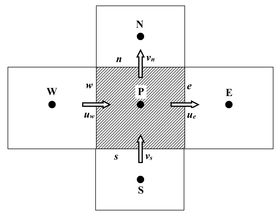
Fig. 26.1 Control point (cell) P and its neighboring cells on a 2D Cartesian grid.#
Eq. (26.1) can be written in discrete form for cell P for a first-order implicit time integration as:
where \(\Omega_P\) is the volume of cell P, and the summation is over all faces f bounding control volume P. The mass flux at any face is given by
where \(\vec{A}\) is the area vector computed at the face centroid.
For the illustrative derivation below, the momentum equation is written as follows:
where \(\boldsymbol{\tau}\) is the viscous stress tensor.
26.1. The SIMPLE algorithm on non-staggered grids#
In this textbook derivation, unstarred variables denote the corrected value produced by one SIMPLE update. They become the final solution only after the nonlinear iterations converge.
The momentum equations given by Eq.(26.4) at the control volume P shown above below can be written, after discretization, as:
In the above equations, the coefficients \(a_*\) result from the discretization procedure – expressions for these coefficients are derived in Chapter 4. For now, suffice it to say that the equations above are discretized versions of the momentum equations which relate the control point P to its neighbors (E, W, N and S). An initial guess for the pressure field \(p^*\) is used to start the solution process. The above equations are solved using the guessed pressure field to yield velocity components \(u^*\) and \(v^*\) as follows:
Next, a correction to pressure, \(p^{'}\), is defined as the difference between the correct pressure field \(p\) and the guessed pressure field \(p^*\), such that:
Similarly, velocity corrections \(u^{\prime}\) and \(v^{\prime}\) are defined to relate the correct velocities \(u\) and \(v\) to the guessed velocities \(u^*\) and \(v^*\), as follows:
Substitution of the correct pressure field \(p\) into the momentum equations yields the correct velocity field \((u, v)\). Subtracting equations (26.1.3) and (26.1.4) from equations (26.1.1) and (26.1.2) respectively, gives:
Using the pressure and velocity decomposition definitions in (26.1.5) and (26.1.6), the above equations can be rewritten as:
At this point, an approximation is introduced: \(\sum a_{\text{nbr}} u_{\text{nbr}}^{\prime} = 0\) and \(\sum a_{\text{nbr}} v_{\text{nbr}}^{\prime} = 0\). This simplifies the equations for the velocity corrections. This is a key approximation unique to the SIMPLE algorithm which yields the following:
where \({}^{(u)}\!C\) and \({}^{(v)}\!C\) are coefficients that depend on the discretization scheme used. The are defined as:
Using Eq. (26.1.6), the velocities can be expressed as
26.1.1. Cell Face Velocities: Momentum Interpolation Technique#
Next, we will illustrate the estimation of control volume interface velocities along the x direction using the so-called momentum interpolation technique (Rhie and Chow[RC83] ). From Eq. (26.1.1), if we assume a uniform mesh and interpolate the pressure at control volume interfaces linearly from the nodal values, the velocities at nodes on either side of the west face can be written as:
which can be written as:
where:
If the velocity at the west face, \(u_w\) , is computed by linearly interpolating \(u_P\) and \(u_W\), we get:
This formulation of interface velocities allows pressure checkerboarding, i.e, it allows odd-even pressure oscillations which are not felt by the velocity field. In order to make the collocated arrangement of velocity and pressure effective, a pressure-velocity coupling mechanism needs to be devised which can suppress the odd-even pressure oscillations. A common approach employed is the so-called momentum interpolation technique. The crux of this technique is to estimate the interface velocity using the momentum equation similar to the nodal momentum equation with the pressure gradient computed using the pressure values at adjacent nodes:
In the above equation, \(\hat{u}_w\) and \(\left( a_P \right)_w\) are computed by interpolating between the adjacent nodal values. Specifically, we use:
Using Eq. (26.1.1.3), we can write the equation above as follows:
The face velocities are designed to be driven by pressure differences between adjacent nodes, not alternate ones. Thus, these velocities are sensitive to checkerboarding and do not allow a checkerboard pressure field. It can be shown that the above expression is equivalent to the following:
Thus, the added dissipation term, which is third-order accurate, does not alter the formal second-order accuracy of the estimation of interface velocities.
To summarize, the momentum interpolation technique provides pressure-velocity coupling via a fourth-derivative pressure dissipation term in the formula for face velocities. Both cell-centered (nodal) and cell face velocities are stored. The nodal velocities satisfy the momentum equations whereas the cell face velocities satisfy mass continuity.
26.1.2. Face Velocity Corrections and Pressure Correction Equation#
Similar to the nodal velocity corrections, the face velocity corrections can be defined as follows:
The corrected face velocities can be written as:
where:
Similar expressions can be derived for \(u_e\) and \(v_e\).
So far, we have only considered the momentum equations but, as mentioned earlier, the velocity field is also subject to the constraint that it should satisfy the continuity equation. Continuity is satisfied in discretized form for the control volume shown in the control volume as:
Substituting the corrected velocities given by Eq. (26.1.2.1) into the discretized continuity equation (26.2), we get:
The above equation can be rearranged as follows:
and can be further re-written as:
where
and the coefficients are given below:
Equation (26.1.2.9) is the equation for pressure correction \(p^{\prime}\) and replaces the discretized continuity equation. It should be noted that we have used primes for the coefficients in Eq. (26.1.2.9) to distinguish them from the coefficients of the discretized momentum equations. The source term \(b^{\prime}\) in the above equation is the continuity imbalance arising from the incorrect velocity field \(u^{*}\), \(v^{*}\). By solving equation (26.1.2.7), the pressure correction field \(p^{\prime}\) can be obtained at all points. Once the pressure correction field is known, the corrected pressure field is obtained using Eq. (26.1.5) and velocity components through the velocity correction equation, Eq. (26.1.6). The omission of terms such as in the derivation does not affect the final solution because the pressure correction and velocity corrections will all be zero in a converged solution giving \(p^{*}= p\), \(u^{*}= u\), and \(v^{*}= v\).
26.1.3. Under-relaxation of Pressure and Velocity#
From the original correction equations, it can be seen that velocity correction consists of two parts: one from the neighboring velocity corrections and the other from the pressure correction field. Dropping the \(\sum a_{nbr} u^{\prime}_nbr\) and \(\sum a_{nbr} v^{\prime}_nbr\) terms places the entire burden of velocity correction on the pressure correction. The pressure correction equation derived with this approximation is susceptible to producing large values of pressure corrections. The corrected velocities always satisfy continuity, regardless of this approximation; however, if the pressure field is updated with the computed pressure correction field it is susceptible to divergence during the course of outer iterations unless some under-relaxation is used during the iterative process. Thus, the pressure values are obtained from the following:
where \(\alpha_P\) is the pressure under-relaxation factor. If we select \(\alpha_p=1\), the guessed pressure field \(p^{*}\) is corrected by \(p^{\prime}\). However, the corrections \(p^{\prime}\), in particular when the guessed field \(p^{*}\) is far away from the final solution, is often too large for stable computations. A value of \(\alpha_P=0\) would imply no correction at all, which is also undesirable. Taking \(\alpha_P\) between 0 and 1 allows us to add to the guessed field \(p^{*}\) a fraction of the correction field \(p^{\prime}\) that is large enough to move the iterative improvement process forward, but small enough to ensure stable computation.
The corrections to the velocity field, however, should not be under-relaxed or else the corrected velocities will not satisfy mass continuity. However, because of non-linearity, it is necessary to under-relax momentum equations while they are being solved using a linear solver. The iteratively improved velocity components \(u^{\text{new}}\) and \(v^{\text{new}}\) are obtained from:
where \(\alpha_u\) and \(\alpha_v\) are the under-relaxation factors for the \(u\) and \(v\) components. These factors have values between 0 and 1. \(u\) and \(v\) are the corrected velocity components without relaxation and \(u^{n-1}\) and \(v^{n-1}\) represent their values obtained in the previous iteration. However, under-relaxation for the velocity field is implemented implicitly in the discretized momentum equations. After some algebra it can be shown that with under-relaxation the discretized \(u\) momentum equation takes the form:
and the discretized v-momentum equation:
It can be observed from the above equations that velocity under-relaxation serves to enhance the diagonal dominance in the coefficient matrix by increasing the magnitude of the central coefficient \(\alpha_P\) by a factor of \(\alpha_u\) and \(\alpha_v\) for \(u\) and \(v\) momentum equations, respectively. The pressure correction equation is also affected by the velocity under-relaxation and it can be shown that the \(C\) terms of the pressure correction equation become:
Note that in these formulae \((a_P)_w\), \((a_P)_e\), \((a_P)_s\) and \((a_P)_n\) are the central coefficients of discretized velocity equations at the west, east, south and north faces of the control volume centered around \(P\), respectively.
A correct choice of under-relaxation factors \(\alpha\) is essential for cost-effective simulations. Too large a value of \(\alpha\) may lead to oscillatory or even divergent iterative solutions and a value which is too small will cause extremely slow convergence. The optimum values of under-relaxation factors are flow dependent.
26.1.4. Outline of the method#
The SIMPLE algorithm gives a method of calculating pressure and velocities. The method is iterative and when other scalars are coupled to the momentum equations, the calculation needs to be conducted sequentially. The sequence of operations in the SIMPLE algorithm is shown below.
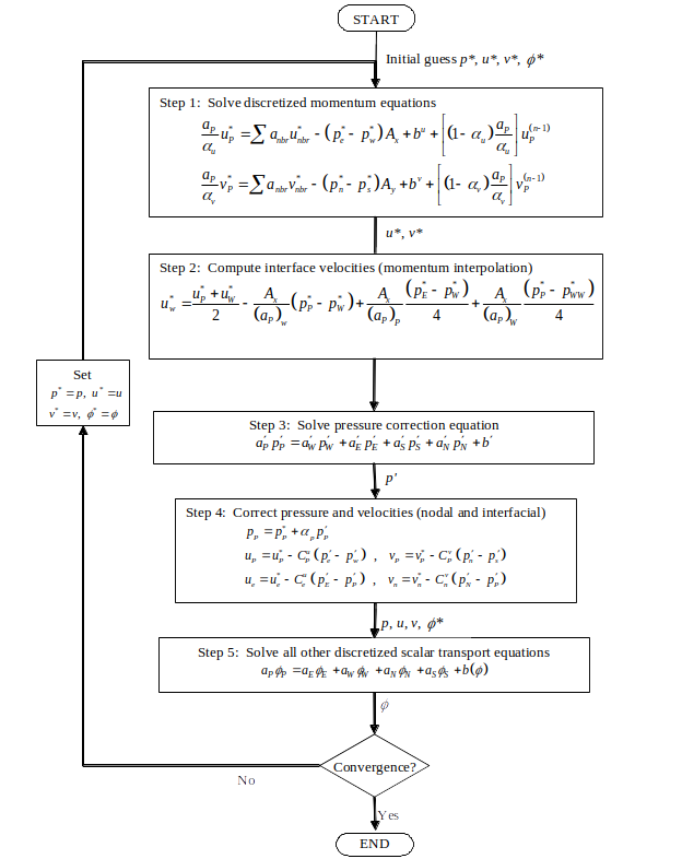
Fig. 26.1.4.1 Sequence of operations in the SIMPLE algorithm.#
26.2. The SIMPLEC algorithm#
The SIMPLEC (SIMPLE-Consistent) algorithm of Van Doormal and Raithby[VDR84] follows the same steps as the SIMPLE algorithm, with the difference that the momentum equations are manipulated so that the SIMPLEC velocity correction equations use an approximation for omitted terms that are less significant than those omitted in SIMPLE.
Note
The equations in this section give the classical steady-grid SIMPLEC derivation and are included to show the origin of the method. Stream uses the same underlying SIMPLEC idea in a collocated unstructured all-speed solver, but with additional momentum-interpolation, unsteady/compressible, and robustness terms in the pressure-correction update. Those additions do not make the method “non-SIMPLEC”; they are implementation refinements of the same SIMPLEC family.
The SIMPLE algorithm neglects the effect of the neighbor velocity corrections, i.e, it uses the following equations for the \(u\) and \(v\) velocity corrections at a node:
The summation term in the equation above is roughly zero in the SIMPLE method. The SIMPLEC algorithm seeks to mitigate the effects of dropping velocity neighbor correction terms. It retains the neighbor velocity correction terms, but approximates them in the following manner:
Thus, the velocity corrections in SIMPLEC are given by:
Similarly, the face velocities can be written as:
where:
Note that momentum under-relaxation is still required in the momentum equations so that the denominator remains finite in the steady limit. The discretized pressure-correction equation has the same general structure as in SIMPLE, except that the \(C\) terms are calculated from Eq. (26.2.7) instead of Eq. (26.1.3.6). The sequence of operations is otherwise identical to that of SIMPLE.
Classically, because the neighbor-correction contribution is retained in approximate form, SIMPLEC often requires less pressure under-relaxation than SIMPLE and usually converges faster. In Stream, pressure-correction relaxation and limiting may still be retained as robustness controls, so the implementation should be viewed as a practical SIMPLEC-family formulation rather than the strict textbook special case.
SIMPLE and SIMPLEC can be shown to be closely related to each other. Recall that pressure correction for SIMPLE is given by:
In the classical steady SIMPLEC derivation, one often writes the pressure update without an additional pressure under-relaxation:
We can think of the SIMPLEC algorithm as solving for a variable \(\bar{p}^{\prime}= \alpha_P p^{\prime}\) and then the pressure correction equation employed by the SIMPLEC algorithm can be written as:
with coefficients of the form:
Recall that the coefficient \(a\) with the prime belongs to the pressure correction equation and those without the prime belong to the momentum equation. Consider the case when \(S_P=0\) for which the central coefficient for the momentum equations is given by:
Thus, neighbor coefficients in the pressure correction equation of the SIMPLEC algorithm are of the following form:
The \(p^{\prime}\) equation for the SIMPLE algorithm is the following:
Multiplying and dividing by \(\alpha_P\) , we can write the above as:
which can be written in terms of \(\bar{p}^{\prime}\) as:
Therefore, we can write:
which can be further written as:
Now, let us compare the coefficients of SIMPLE and SIMPLEC. If we choose:
in the classical steady-grid SIMPLE algorithm, we would effectively get the same corrected pressure each iteration for both SIMPLE and SIMPLEC. With this viewpoint, it can be seen that the two algorithms are closely related. If one uses the SIMPLE algorithm with \(\alpha_P = 1 - \alpha_u\), then the classical textbook update resembles SIMPLEC when \(S_P=0\). Stream retains this same basic SIMPLEC idea, while using implementation-specific coefficient and correction forms suited to the all-speed collocated solver.
26.3. References#
C.L. Rhie and W.L. Chow. A numerical study of the turbulent flow past an isolated airfoil with trailing edge separation. AIAA Journal, 21:1525–1532, 1983.
J.P. Van Doormaal and G.D. Raithby. Enhancements of the simple method for predicting incompressible fluid flows. Numerical Heat Transfer, 7(2):147–163, 1984. URL: https://www.tandfonline.com/doi/abs/10.1080/01495728408961817, doi:10.1080/01495728408961817.