4. Finite-Volume Transport Assembly on Unstructured Grids#
This chapter derives how the conservation laws become discrete finite-volume transport equations on an unstructured grid. Chapter 3 supplied the algorithmic map; the present chapter develops the temporal, convective, diffusive, pressure-gradient, and source contributions that form each transported algebraic row. The momentum-weighted face-flux construction is developed in Chapter 5, and the pressure-correction row is developed in Chapter 6.
A compact state picture of the solution process is:
Here \(n\) denotes the previous converged time level, while \(k\) and \(k+1\) denote successive outer-iteration states at the new time level. The purpose of this chapter is narrower than the complete sequence shown above: it freezes the current coefficients and asks how one conservation law becomes one sparse algebraic row. The provisional face flux and pressure-correction equation that couple those rows are developed in Chapter 5 and Chapter 6, respectively.
For reference, the continuous continuity equation is
To keep the assembly formulas readable, most derivations in this chapter are written with a first-order implicit Euler (BDF1) time discretization. When other time schemes change the diagonal, neighbor, or right-hand-side terms, that dependence is stated explicitly, but the full discussion of higher-order temporal integration is deferred to Chapter 10. For integration in space, Green’s theorem is used to convert the volume integral to a surface integral. Consider a control volume (cell) labeled \(P\) in the figure below. This volume is bounded by a finite number of faces.
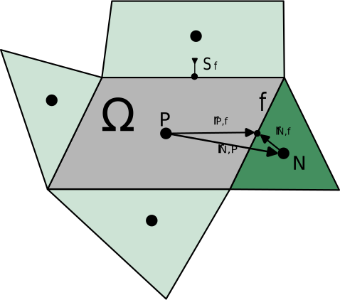
Fig. 4.1 Control volume \(P\) and neighboring cell \(N\) for integration on a 2D unstructured grid.#
In the diagram above, the \(Omega\) is the volume of the control volume \(P\), the vector \(r_{P,f}\) is the vector pointing from the centroid of cell \(P\) to the centroid of face \(f\). The vector \(S_f\) is an area vector pointing in the same direction as the face \(f\)’s unit normal vector a magnitude equal to the area of that face i.e. \(\vec{S}_f = A_f \cdot \vec{n}_f\) where \(\vec{n}_f\) is the unit vector for face \(f\). The orientation of this vector may be into cell P or out of cell P, depending on however the unit normal vectors are defined for the faces that make up cell \(P\).
We will use calligraphic symbols to name collections of mesh entities, and \(\in\) means “is one of.” The face and neighbor vocabulary is:
\(\mathcal F_P\) is the collection of faces of cell \(P\). Thus an expression like \(f\in\mathcal F_P\) means that \(f\) is one of the faces of the set of all faces that belong to cell \(P\).
Considering the faces of cell \(P\) (\(f\in\mathcal F_P\)), we defined \(N_f\) to mean the cell on the other side of face \(f\).
\(\mathcal N(P)\) is the collection of distinct neighboring cells reached through those faces of \(P\). Thus \(N\in\mathcal N(P)\) means that \(N\) is one of the cell-centered neighbors of \(P\).
\(\mathcal F(P,N)\) is the collection of faces connecting the particular cell pair \(P\) and \(N\).
Accordingly, \(\sum_{f\in\mathcal F_P}\) means “add one contribution for every face of \(P\)”, and \(\sum_{N\in\mathcal N(P)}\) means “add one contribution for every distinct neighboring cell,” and \(\sum_{f\in\mathcal F(P,N)}\) means “add the contributions from every face connecting \(P\) and \(N\).” Every face has one cell \(N_f\) on its other side, but two cells may be connected by more than one face. Face contributions are therefore assembled face by face and then collected into one matrix coefficient for each distinct neighbor \(N\). An unqualified \(\sum_f\) means “add one contribution for every face bounding \(P\)” and therefore includes physical boundary faces as well as internal faces.
The derivations in this chapter consider an cell with internal faces surrounding it. A physical boundary face replaces the corresponding two-cell term through a one-sided relation developed in the boundary-condition subsection; boundary terms are not carried through every step of the internal-face algebra.
The continuity equation above can be written in discrete form for cell \(P\) as:
where \(\Omega_P\) is the volume of cell \(P\), and the summation is over all faces \(f\) bounding control volume \(P\). The mass flux at any face is given by
where \(\vec{A}\) is the area vector computed at the face centroid.
The high-level goal is to assemble each transported equation into a row of the form
The parenthesized left prescript in the above equation identifies the equation or construction to which a symbol belongs. Thus \({}^{(\phi)}\!a_P\) is the central coefficient of the \(\phi\) equation.
4.1. Algebraic Form of the Cell Equation#
Throughout this guide, there are canonical algebraic forms of governing equations that are worth understanding. This form of equation is used when deriving the generic transported-component equation used for velocity components, energy, species, turbulence quantities, and similar transported unknowns. Below is the general form of this equation.
This chapter focuses on the derivation of the transport equation’s version of this equation and the meaning of its coefficients. Sometimes this may be called a Row Equation or a Row-Form Equation. As you can see from the subscript \(P\), this equation is associated with the control volume of a generic cell \(P\). The accumulation of all of of the equations for all the cells in a domain forms a sparse matrix system that is solved to advance the solution. So each cell’s algebraic equation is inserted as one of the rows of the linear algebra matrix system, thus the name Row Equation. This process of putting together this algebraic equation is also often called assembly of the row equation.
If several faces connect \(P\) to the same \(N\), they contribute several terms to the face sum but only one aggregated coefficient \({}^{(\phi)}\!a_{P,N}\) in the neighbor sum. For boundary-face quantities, we use the subscript \(\mathrm{bnd}\). When a sum over boundary faces of cell \(P\) is needed, the notation \(\sum_{\text{bnd}}\) is used. If only one class of boundary faces contributes, that qualifier is attached directly to the sum; for example, \(\sum_{\text{bnd}^{(p)}}\) denotes a sum over the specified-pressure boundary faces of cell \(P\).
One important distinction to keep in mind is that some approximations may use information from a wider reconstruction or gradient stencil. Those extra cells are not members of \(\mathcal N(P)\) merely because they enter a reconstruction. When wider-stencil information is used, the effect of that larger collection of cells is usually kept explicit and collected into source-like correction terms in \({}^{(\phi)}\!b_P\). The implicit row therefore continues to involve only the cells directly connected to \(P\) through an internal face. In other words, if you examine the matrix row for cell \(P\), you will only see nonzero entries for the diagonal and the immediately adjacent neighbors \(N\in\mathcal N(P)\). The effect that those other cell’s contribution to the row equation is relegated to the explicit source term \({}^{(\phi)}\!b_P\).
The coefficient bookkeeping is handled in a way that the final coefficients of that algebraic equation above can be thought of as sums of various different types of contributions that arise due to different terms in the equation or different ways of discretizing the terms. For a generic transport equation, the row equation’s the final stored coefficients are built by collecting the contribution from each of the various pieces. Some of these common pieces are the contributions to the equation from the convective terms, the diffusive terms, the temporal terms, and source terms for example. Below shows for example how each of the primary coefficients is assembled as a sum of the elements that make it up.
The same bookkeeping can also be used to group the elements that make up the main coefficients into temporal and spatial contributions.
The boxed summaries throughout this chapter are the pieces added together to form the final \({}^{(\phi)}\!a_P\), \({}^{(\phi)}\!a_{\text{nbr}}\), and \({}^{(\phi)}\!b_P\) of the transported row. These are just a quick reference for what each of the pieces are and what they contribute to the final result of the coefficients of the algebraic row equation.
4.2. Decomposition of Generic Transport Equation to Algebraic Cell Equation#
This section shows how the common form of a transport equation is turned into the algebraic row equation used by Stream. For a true generic scalar equations that have the form of the equation shown below, such as energy, species, and turbulence transport, this template applies directly. Each component of the momentum equation can also be written in an analogous row form, but the pressure term and viscous-stress contributions require additional treatment that will be discussed after the generic equation is handled.
Consider a generic scalar transport equation like the one shown below.
where \(\phi\) can stand for one transported component such as \(u\), \(v\), \(w\), \(H\), \(Y_k\), \(k\), or \(\omega\). The equation above is the common template for a single transported unknown. The terms labeled in the equation above are:
(1) Unsteady: the time-derivative contribution.
(2) Convection: the advective flux divergence.
(3) Diffusion: the diffusive flux divergence.
(4) Source terms: any remaining contributions not captured by the above three.
Integrating the transport equation over control volume (P) and applying Gauss’s divergence theorem converts the convective and diffusive divergence terms into fluxes across the cell faces. The exact control-volume integral balance is:
Writing the boundary integral as a sum of face integrals is an exact partition of the boundary. It is not yet a spatial discretization. It becomes semi-discrete when those integrals are approximated using the finite set of cell and face values as shown below.
Here, the volume integrals have been replaced by cell-average quadrature and the face integrals by numerical face fluxes. Space is therefore discrete, while time remains continuous.
The main components of the discretization procedure for the above equation are:
Discretization of the convection terms
Discretization of the diffusion terms
Estimation of the mass flux at control volume faces
The discretization, to be described in the following sections, leads to an algebraic equation for each control volume which can be written as:
This is still semi-discrete. It is a further assembly or linearization of the spatially discrete operator. The subscript spatial means that the convection, diffusion, and spatial source pieces have been collected while the transient storage term is still displayed separately. In particular, \({}^{(\phi)}\!a_{P,N,\mathrm{spatial}}\) contains the contributions from every face in \(\mathcal F(P,N)\).
Once the temporal term is discretized in time and its contributions are written in the same algebraic form as the spatial terms, the equation will have form introduced above, with \({}^{(\phi)}\!a_P\) as the final central coefficient, \({}^{(\phi)}\!a_{P,N}\) as the final implicit coupling to neighbor \(N\), and \({}^{(\phi)}\!b_P\) as the final discrete source term.
One conceptual distinction here that is relevant to Stream is that it assembles the equations for the rows by sweeping over all the faces and adding the face terms to the cells on either side of a face. So instead of the equation being assembled by considering a cell and looping over all faces of that cell and writing the algebraic equation, you could loop over all faces in a domain and then update the cell equations for the cells that are adjacent to each face. And once again, because this is a generic finite volume cell solver where two cells can share multiple faces, contributions from multiple faces connecting the same two cells accumulate in the same \({}^{(\phi)}\!a_{P,N}\) entry.
4.2.1. Diffusion Terms#
In the generic transport equation, Eq. (4.2.1), the diffusion operator is
For one control volume \(P\), the first step is to integrate that operator over the cell volume \(\Omega_P\).
Using the divergence theorem, \(\int_{\Omega_P} \nabla \cdot (\Gamma \nabla \phi)\, d\Omega = \int_{\partial \Omega_P} \Gamma \nabla \phi \cdot \hat{\vec{n}}\, dA\), so the volume integral becomes a net diffusive flux through the cell boundary.
As discussed earlier, in the standard finite-volume discretization, that boundary integral is approximated by summing the flux through each face of the control volume. This is why the discrete diffusion contribution naturally appears as a face sum rather than as a cell-centered Laplacian:
Here \(D_f\) is simply a shorthand for the diffusive contribution coming through face \(f\) i.e.
To obtain matrix coefficients, each face contribution must be written in terms of the unknowns stored at the two cells that are adjacent to that face, namely \(P\) and \(N\). First, introduce the center-to-center vector from cell \(P\) to cell \(N\),
Along that line, the directional derivative is approximated by the two-point difference
The motivation for using this simple approximation is to build an implicit matrix row with a small, local stencil: ideally one diagonal contribution for cell \(P\) and one neighbor contribution for cell \(N\) from each face. The two-point difference above does exactly that, because it depends only on the immediately adjacent cell values \(\phi_P\) and \(\phi_N\). A wider-stencil or higher-order reconstructed face gradient could certainly be used to improve the estimate of \((\nabla \phi)_f\), but if that information were kept fully implicit it would generally enlarge the stencil and complicate the matrix coefficients. The choice made here is therefore: keep the center-to-center derivative simple and local in the implicit operator, and treat the remaining non-orthogonal part as an explicit correction. This is in essence keeping the part of that gradient that is aligned between the cell centers and relegating the rest of that quantity to show up as an explicit source term in the final algebraic equation for the row equation.
The geometric issue is that the derivative we can approximate implicitly with neighboring cell values is the derivative along \(\hat{\vec{r}}_{PN}\), while the flux requires the derivative contracted with the face-area vector \(\vec{A}_f\). On an orthogonal mesh those directions are aligned. On a skewed mesh they are not. Figure Fig. 4.2.1.1 shows this mismatch for one internal face.
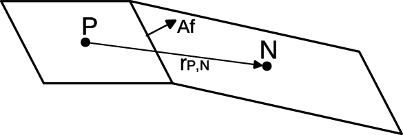
Fig. 4.2.1.1 Non-orthogonal geometry at the face shared by cells \(P\) and \(N\). The center-to-center vector \(\vec{r}_{PN}\) is not parallel to the face-area vector \(\vec{A}_f\).#
To keep the implicit part aligned with the compact \(P\)–\(N\) stencil, decompose the face-area vector into two vectors:
We define \(\vec{E}_f\) to be the part that is parallel to the vector connecting the cell centers, \(\hat{\vec{r}}_{PN}\) .
This leaves the remainder \(\vec{T}_f\) as the part of the original face area vector that is not carried by the center-to-center aligned contribution \(\vec{E}_f\).
Here, we choose what is called the over-relaxed decomposition, which means that \(\alpha_f\) is not the ordinary projection of \(\vec{A}_f\) onto \(\hat{\vec{r}}_{PN}\). Instead, it is chosen so that the remainder \(\vec{T}_f\) is tangent to the face. Consequently, the centerline-aligned vector \(\vec{E}_f\) carries the complete face-normal area contribution, while \(\vec{T}_f\) supplies a tangential non-orthogonal correction. This is not the minimum-magnitude decomposition of \(\vec{A}_f\); that distinction is why it is called over-relaxed. Figure Fig. 4.2.1.2 shows the resulting vector geometry.
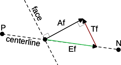
Fig. 4.2.1.2 Over-relaxed decomposition of the face-area vector. The vector \(\vec{E}_f\) is parallel to \(\vec{r}_{PN}\), while \(\vec{T}_f=\vec{A}_f-\vec{E}_f\) is tangent to the face. Consequently, \(\vec{T}_f\cdot\vec{A}_f=0\).#
The tangency condition is
We can get the value of \(\alpha_f\) that makes this condition true by substituting \(\vec{T}_f = \vec{A}_f - \alpha_f \hat{\vec{r}}_{PN}\) into that equation:
Solving for \(\alpha_f\) gives:
The decomposition of the face area vector into the aligned part \(\vec{E}_f\) and the tangential correction \(\vec{T}_f\) is therefore:
Over-Relaxed Decomposition Step
With the centerline-aligned part being \(\vec{E}_f\), and the tangential part being \(\vec{T}_f\)
With that notation, substituting Eq. (4.2.1.13) into Eq. (4.2.1.4) gives the exact split
The two flux contributions correspond to the centerline-aligned and tangential directions shown in Figure Fig. 4.2.1.2.
Now the two-point approximation can be substituted directly into the directional derivative along \(\hat{\vec{r}}_{PN}\):
That covers the aligned part of the flux, but the remaining face gradient in the correction term still needs to be approximated so as to not have any unknowns at the face. The choice made here is to use a lagged face gradient \(\overline{\nabla \phi}_f\) that is estimated from the neighboring cell-centered gradients. This means that the correction term will be treated explicitly as part of the source term \(b_P\) rather than being fed into the matrix coefficients.
Final Scalar Diffusion Flux Split
With those two approximations, the face diffusion flux is
The first term is the compact implicit contribution built from the local \(P\)–\(N\) stencil, while the second term is the explicit non-orthogonal correction.
Assumptions In This Split
Two different approximations are being made here, and they are intentionally not the same.
For the aligned part, we use the two-point directional derivative \(\;(\nabla \phi)_f \cdot \hat{\vec{r}}_{PN} \approx (\phi_N - \phi_P)/d_{PN}\;\), because this keeps the implicit matrix contribution local to the \(P\)–\(N\) stencil.
For the correction part, we do not apply the same two-point approximation, because that difference only approximates the derivative along the center-to-center direction, not the leftover tangential direction carried by \(\vec{T}_f\). Instead, that term is treated explicitly with a lagged face-gradient estimate.
In practice, \(\overline{\nabla \phi}_f\) should be read as an approximation to the gradient field at the face obtained from the neighboring cell-centered gradients. In the simplest form used in this discussion,
So the second term is still approximate; it is just approximate in a different way. The first term gives the compact implicit diffusion coefficient, while the second term carries the non-orthogonal correction explicitly.
When The Field Is Not Smooth
The discussion above assumes that the gradient field is smooth enough that a face-gradient estimate such as \(\overline{\nabla \phi}_f\) is meaningful. When \(\phi\) has a sharp jump, when the mesh under-resolves a thin layer, or when the diffusivity changes abruptly across the face, that assumption becomes weaker and the explicit non-orthogonal correction can become noisy or overly aggressive.
Common remedies in such situations are:
reduce or suppress the non-orthogonal correction locally and rely more heavily on the compact two-point implicit term;
limit the reconstructed cell-centered gradients before forming \(\overline{\nabla \phi}_f\);
use a more appropriate face diffusivity, such as a harmonic average, when the coefficient \(\Gamma\) itself changes abruptly;
for genuine material interfaces or other true discontinuities, replace the simple averaged face-gradient model with a one-sided or interface-aware treatment.
The main point is that the compact split derived above is most reliable when the field is reasonably smooth over the \(P\)–\(N\) stencil. Near strong jumps, extra limiting or interface modeling may be needed for robustness.
Introduce the compact face coefficient
Then Eq. (4.2.1.16) can be written as
Here we can see that the face diffusion flux has been split into a part multiplying the current-cell unknown \(\phi_P\), a part multiplying the neighbor unknown \(\phi_N\), and a remainder that is treated explicitly. This is the final form of this term, and from this we can express this equation in that standard algebraic form that we have discussed previously.
Final Standard Diffusive Row Contribution
After summing the face contributions for cell \(P\) and rearranging them into the row form of Eq. (4.2.3), the diffusive part of the row equation. These are the diffusion pieces that will be added to the full row coefficients \({}^{(\phi)}\!a_P\), \({}^{(\phi)}\!a_{P,N}\), and \({}^{(\phi)}\!b_P\).
with
and
4.2.1.1. Additional Terms For Momentum Diffusion#
For scalar equations such as energy, species, and turbulence transport, the diffusion discussion above is the whole story: the diffusive flux is just the generic term in Eq. (4.2.1.3). The momentum equations, on the other hand, contain additional viscous-stress terms beyond that generic scalar form. This section covers how those extra momentum-specific terms manifest. The viscous contribution is written as:
where \(\Gamma = \mu + \mu_t\) and \(\mathbf{I}\) is the identity tensor. Here \(\mu\) is the molecular (laminar) dynamic viscosity, while \(\mu_t\) is the turbulent or eddy viscosity supplied by the turbulence model. In a laminar calculation, \(\mu_t = 0\), so \(\Gamma\) reduces to the physical viscosity \(\mu\) alone. It is convenient to split this into a Laplacian-like part and a remaining viscous-stress correction:
After integrating over the control volume, the first term becomes
which is just the vector analogue of the generic diffusion term in Eq. (4.2.1.3), applied componentwise to the velocity field. The second term in Eq. (4.2.1.26) becomes the expression below.
This term is treated explicitly as part of the momentum source term. This means that \((\nabla \vec{u})_f\) and \((\nabla \cdot \vec{u})_f\) are not introduced as additional face unknowns in the implicit system. Instead, they are reconstructed from the cell-centered velocity-gradient field and then interpolated to the face in a lagged manner. At the level of this derivation, one can think of interior-face estimates such as
with the understanding that the exact interpolation and boundary treatment are implementation details. The important point is that this second viscous term is handled explicitly from reconstructed gradients, whereas the compact \(\nabla \cdot (\Gamma \nabla \vec{u})\) part is the part kept in the local implicit stencil. When the solver assembles one momentum-component row, it simply takes the corresponding component of these vector expressions.
That means an algebraic row can be written for the diffusion part of one momentum component just as it was for a generic transported scalar. If we denote by \(u_i\) the selected velocity component, then the compact Laplacian-like part contributes exactly the same kind of local \(P\)–\(N\) coefficient as before, now with \(\phi = u_i\). The extra viscous-stress piece contributes only to the explicit source because it is reconstructed from lagged gradients rather than implicitized as additional face unknowns.
For one interior face shared by cells \(P\) and \(N\), the diffusive contribution to the \(i\)th momentum-component row separates into three parts:
Here \(\mathcal K_f\) is the compact coefficient defined in the generic diffusion derivation with \(\phi=u_i\). The other two terms are evaluated explicitly from reconstructed gradients.
Final Momentum-Diffusion Row Contribution
For one velocity component \(u_i\), the diffusive part of the assembled momentum row is
with
So the bookkeeping is the same as before:
the Laplacian-like part feeds the diagonal and neighbor coefficients,
the non-orthogonal diffusion correction stays in the explicit source,
and the extra viscous-stress term also stays in the explicit source.
Smoothness Caveat For The Viscous-Stress Correction
This explicit viscous-stress correction inherits the same kind of smooth-field assumption as the earlier non-orthogonal diffusion correction. Its accuracy depends on the reconstructed velocity-gradient field being smooth enough that face estimates of \((\nabla \vec{u})_f\) and \((\nabla \cdot \vec{u})_f\) are meaningful.
The relevant warning sign here is a sharp variation or unresolved jump in the velocity field, if velocity or viscosity changes abruptly across a short distance, the reconstructed gradients can become noisy and the explicit correction can be too aggressive.
In such situations, the same kinds of remedies discussed above may be needed: limiting the reconstructed gradients, damping the explicit correction, or using more specialized interface-aware treatment when a true discontinuity is present.
4.2.2. Convection Terms#
We now turn to the convective face flux that appears in Eq. (4.2.3). We therefore begin at that generic level, where \(\phi\) denotes an arbitrary transported variable and the algebra applies equally to energy, species, turbulence variables, or one component of velocity. The pressure-gradient term is not part of convection, so it is handled separately in the next section.
For ease of illustration, the convection discussion below uses an upwind scheme for the transported primitive variable. When we return to the momentum-specific pressure term, we use a central-difference treatment for that separate contribution. Upwind schemes are commonly employed for incompressible flows. They can also be employed for compressible flows, though characteristics-based methods are usually more appropriate for compressible flows; those are described in Chapter 9.
For cell \(P\), the discrete convection contribution that appears in Eq. (4.2.3) is the face sum below.
Each face contributes one term \(\dot{m}_f \phi_f\) to the cell equation. The final result of this section is to show how you go from the above form to the final algebraic form below that is composed of main coefficients, neighbor coefficients, and explicit source terms.
While discretizing this convection term, the mass flux \(\dot{m}_f\) is assumed to be known and is considered positive along the direction of the face normal pointing away from cell \(P\) (and towards cell \(N\)). Thus, the convective flux at any face is given by \(\dot{m}_f \phi_f\) where the face value of the transported variable \(\phi_f\) is obtained by upwinding based on the sign of the mass flux:
where \(\phi_{f,P}\) and \(\phi_{f,N}\) are the what we can call candidate face values at face \(f\) reconstructed from cells \(P\) and \(N\), respectively. In other words, the notation means “the value supplied to face \(f\) from the \(P\) side” and “the value supplied to face \(f\) from the \(N\) side.” This notation is intentionally generic: for a first-order upwind scheme, no reconstruction is used, so these reduce to the adjacent cell values \(\phi_{f,P}=\phi_P\) and \(\phi_{f,N}=\phi_N\); for a second-order upwind-type reconstruction, they are the reconstructed values obtained from the cell-centered gradients. The actual face value \(\phi_f\) is then whichever of these two candidate values lies on the upwind side of the face.
We have not used a split-flux notation earlier in the guide, so we introduce it here for convenience. Define the positive and negative parts of the face mass flux by
so that both \(\dot{m}_f^{+}\) and \(\dot{m}_f^{-}\) are nonnegative magnitudes. With these definitions, the convective face flux for a face can be written in the generic split form
This split form is simply a compact algebraic way to encode the sign-based donor-cell choice without writing a case distinction for every face. If \(\dot{m}_f>0\), then \(\dot{m}_f^{+}=\dot{m}_f\) and \(\dot{m}_f^{-}=0\), so the flux reduces to \(\dot{m}_f\phi_{f,P}\). If \(\dot{m}_f<0\), then \(\dot{m}_f^{+}=0\) and \(\dot{m}_f^{-}=-\dot{m}_f\), so the same expression reduces to \(\dot{m}_f\phi_{f,N}\).
The notation is useful because it makes matrix assembly much easier to read. Once the flux is written in split form, the coefficient multiplying \(\phi_P\) can be identified immediately as part of the diagonal contribution, while the coefficient multiplying \(\phi_N\) is the neighbor contribution.
To construct a second-order scheme, a linear reconstruction procedure is adopted for computing the candidate face values \(\phi_{f,P}\) and \(\phi_{f,N}\) by using the gradient of \(\phi\) computed at the cell centers. The gradient reconstruction operator is modified by using a limiter (\(\Psi\)) in order to avoid any local extrema. The final expressions are as follows:
where \( \vec{dr} \) is the vector from the centroid of the cell to the centroid of the face. Two limiters are used, namely, those proposed by Barth and its modification proposed by Venkatakrishnan. For cell \(P\), the Barth limiter is computed as follows:
first compute \(\phi_P^{\min}=\min(\phi_P,\phi_{\text{neighbors}})\) and \(\phi_P^{\max}=\max(\phi_P,\phi_{\text{neighbors}})\)
next, each vertex i of the cell, compute \(\phi_i\) using the equation above with \(\Psi\) set to 1.
then, compute:
finally, compute \(\Psi_P=\min(\bar{\Psi}_{Pi})\), where \(i=1,\ldots,NV_P\) and \(NV_P\) is the number of vertices in cell \(P\).
Similarly, one can compute the limiter function \(\Psi_N\) for cell \(N\). Substituting these reconstructed candidate values into the generic split-flux form gives
Separating the first-order part from the reconstruction increment gives
If we define \(\phi_f^{(1)}\) as the selected first-order face value and collect the higher-order reconstruction increment into
then the facewise convective flux can be written as
This is the key algebraic split for convection. The first term is the compact first-order upwind operator, and the second term is the reconstruction increment that upgrades that first-order face value to the selected higher-order face value. For a first-order scheme, \(\delta \phi_f^{(2)} = 0\) and only the compact upwind term remains.
Summing the facewise identity over the internal-face prototype gives
For the generic transported-variable row in Eq. (4.2.3), this already shows how convection enters the algebraic form in the direct split-flux view: for one interior face \(f\), the first-order part contributes \(\dot{m}_f^{+}\) to the coefficient multiplying \(\phi_P\), contributes \(\dot{m}_f^{-}\) to the coefficient multiplying \(\phi_N\), and contributes \(-\dot{m}_f \, \delta \phi_f^{(2)}\) as an explicit source term. This correction is treated as a source term because, in the linear solve, it is evaluated from lagged reconstructed gradients and limiters rather than being implicitized as part of the compact local \(P\)–\(N\) stencil. If it were kept fully implicit, the coefficients would depend not only on \(\phi_P\) and \(\phi_N\) but also on the wider set of cells entering the reconstructed gradients and limiter values.
Final Standard Convective Row Contribution
For the direct split-flux form of Eq. (4.2.3), the convective contribution is
with
So in the direct form, the outgoing first-order flux feeds the diagonal, the incoming first-order flux feeds the neighbor coefficient, and the higher-order reconstruction increment remains explicit.
A commonly used variation of the convective discretization is to subtract \(\phi_P\) times the discrete continuity equation from the transport row. This does not change the converged equation when discrete continuity is satisfied, but it reshuffles the algebra in a way that is often helpful for diagonal dominance and linear-solver robustness. The continuity equation used here is the same cellwise balance already written in Eq. (4.3), i.e. the continuity equation after integration over control volume \(P\) and replacement of the surface integral by the face-flux sum. Written before any terms are dropped or regrouped, that operation is
At the semi-discrete level, the operation can be shown before choosing BDF1, BDF2, or another time-integration scheme:
Grouping the temporal and face terms gives
Applying the temporal product rule then produces
This exposes the change in the convection term directly:
If mass transfer is present, the semi-discrete continuity equation is
and the corresponding source-aware transport form is
We can move some terms around to get to a form that looks similar to the canonical transport template in Eq. (4.2.3):
The reason for writing it this way is that the subtracted bracket is exactly zero when discrete continuity is satisfied, so this does not change the converged equation; it only changes how the convective and unsteady pieces are arranged during the linear solve. We are not throwing away the rest of the transport row. Diffusion and other explicit source terms are untouched by this particular manipulation, because they are not part of the continuity equation. The unsteady term is also affected by the same continuity-added operation, but its bookkeeping belongs with the temporal coefficient assembly rather than with the face-by-face convection algebra. In the discussion just below, we therefore focus only on the convection part of that altered equation and how that reshuffling changes the algebraic form of the convective contribution to the row coefficients. Focusing on that second term in brackets, we see that it bears the same resemblance to the original convection term with an extra subtraction:
If continuity contains a mass source, the same idea applies, but the subtracted continuity balance must include that source. In residual form, the quantity multiplied by \(\phi_P\) is then
Thus the continuity-added manipulation remains an algebraic rewrite of the same converged equation when particle mass transfer or another mass source is active. Any apparent \(+\phi S_{\rho}\) term introduced by writing a specific-variable equation with a conservative \(\rho\phi\) left-hand side is canceled by the corresponding \(-\phi S_{\rho}\) contribution from the full continuity residual. The physical model source \(S_{\rho\phi}\) itself is not canceled. The source-aware continuum bookkeeping is summarized in the detailed governing-equations appendix.
We know how that first term can be written from (4.2.2.12), and we know the definition of the split mass flux from (4.2.2.4), so the internal-face portion of the continuity-added convection contribution is
A little algebraic manipulation gives
The first two terms cancel, leaving
The continuity subtraction reorganizes only the first-order part. The higher-order reconstruction term \(\sum_{f\in\mathcal F_P}\dot m_f\,\delta\phi_f^{(2)}\) carries through unchanged.
Final Continuity-Added Convective Row Contribution
For the continuity-added form of the same transport template, the convective contribution is
with
So the continuity subtraction reshuffles only the first-order part of the convective operator: the inflow contribution becomes the implicit backbone, while the higher-order reconstruction term remains explicit in the source.
4.2.3. Pressure Contribution in the Momentum Row#
Unlike the diffusion and convection terms discussed above, pressure does not appear in the generic transported-scalar row of Eq. (4.2.3). It enters only after we specialize \(\phi\) to the momentum equation. Written in the same semi-discrete control-volume style used for the scalar transport equation, the momentum balance for cell \(P\) is
This is the vector analogue of Eq. (4.2.3): the transient and convective terms look the same in structure, the viscous contribution is gathered into the face sum \(\sum_f \vec{D}_f\), and the momentum equation carries one extra term that the generic scalar row does not, namely the pressure-gradient contribution. Here \(\vec{D}_f\) denotes the total viscous face contribution, including both the Laplacian-like diffusion part and the additional momentum-specific viscous-stress correction discussed in the previous subsection.
The pressure term we are concerned with in this section is therefore the control-volume pressure contribution. Define
This contribution can be discretized in two closely related ways. If it is treated as a volume term built from the cell-centered pressure gradient, then
In plain language, this first form says: estimate one pressure-gradient vector at the cell center, and use that single vector to represent the pressure force over the whole control volume. It does not mean that pressure is assumed constant in the cell. Rather, it means that the integrated pressure-force term is approximated from a cell-centered gradient estimate. This is the form used in the momentum relation employed for face-mass-flux construction in the next subsection.
The same contribution can also be written in surface-integral form by starting from the continuous \(-\nabla p\) term in the momentum equation and applying Green’s theorem over cell \(P\):
In this second form, the pressure contribution is viewed as the sum of the pressure forces acting on the cell faces. So the discrete data now live at the faces: one estimates a pressure value \(p_f\) on each face, multiplies by the face area vector, and sums those contributions around the control volume.
So the conceptual difference is:
Cell-centered gradient form: one gradient vector per cell, used to approximate the integrated pressure force.
Face-based form: one pressure estimate per face, used to build the integrated pressure force as a sum of face contributions.
In the continuous equations these are equivalent descriptions of the same term. Discretely, however, they are not identical, because one relies on a cell-centered gradient reconstruction while the other relies on face-pressure estimates. In both cases, it is this quantity \(\mathcal{P}_{P,i}\) that appears with a minus sign in the integrated momentum balance of Eq. (4.2.3.1).
4.2.3.1. Face Flux Supplied by Momentum Interpolation#
For each velocity component, the collected momentum row has the same \({}^{(u)}\!a_P\), \({}^{(u)}\!a_{P,N}\), and \({}^{(u)}\!b_{P,i}\) structure as the scalar row, with \(-\mathcal P_{P,i}\) included in its known RHS. Equation (5.3.1.7) expands that RHS into its time, convection, viscous, physical-source, and pressure pieces before constructing the face flux. This keeps the cell assembly and interpolation coefficient definitions connected.
The assembled cell momentum equation supplies a provisional cell-centered velocity, but continuity is evaluated from face fluxes. On a collocated grid, those fluxes require a pressure-coupled construction rather than a plain interpolation of the cell velocities. The complete unstructured derivation, including the classical Rhie–Chow/Majumdar form, time-consistent Pascau and Choi forms, source-balanced corrections, and the Denner form, is given in Chapter 5.
For the subsequent pressure-correction assembly, momentum interpolation has two outputs:
the known provisional face flux \(\hat m_f^*\), including its transport, pressure, relaxation, time-history, geometry, and source-balance contributions; and
a positive face pressure-response coefficient \(d_f\) such that the pressure-induced flux correction is linear in the pressure-correction difference across the face.
When a momentum source contributes a scalar coefficient to the implicit diagonal, momentum interpolation uses the resulting assembled diagonal. The porous-media appendix develops this coupling for a resistance source.
The selected interpolation changes the formulas used to construct \(\hat m_f^*\) and \(d_f\). Once those two quantities have been supplied, the continuity linearization and sparse pressure-correction row follow the same assembly pattern for every interpolation family.