9. High-Resolution Schemes for Compressible Flows

In order to accurately predict surface pressure and heat transfer rates in inviscid and viscous compressible flows in an all-speed manner, robust and accurate numerical schemes are required for solving the governing equations. Schemes such as the standard first-order upwind scheme can provide robust solutions for a broad range of flows, but they are not accurate enough in the presence of strong discontinuities such as shock waves. The standard second-order upwind schemes provide relatively accurate results for smooth inviscid and viscous flows, but can cause spurious oscillations near shocks. To remedy these deficiencies, compressible, characteristic-based convection schemes such as AUSM\(^+\)-up, SLAU and SLAU2 schemes have been implemented in Loci-STREAM. These schemes are robust and accurate for inviscid and viscous compressible flows and allow simulations to be performed in an all-speed manner. The AUSM\(^+\)-up scheme and the SLAU2 scheme are robust for flows at all Mach numbers and are relatively simple and accurate. The SLAU2 scheme requires special treatment in unstructured grids to cure the carbuncle phenomenon, which manifests as odd-even decoupling on the shock profile. The hybrid-SLAU2 scheme is designed to resolve the carbuncle phenomenon in hypersonic flows on unstructured grids. The convergence properties of different convection schemes and limiters are examined for a variety of test cases.

9.1. AUSM±up for Unstructured Grids

The AUSM\(^+\) scheme, originally developed by Liou [38], is an improvement over the earlier AUSM scheme developed by Liou and Steffen [39]. Like AUSM, AUSM\(^+\) is based on splitting of inviscid fluxes into convective and pressure parts. The improvement in AUSM\(^+\) is in the Mach-number based splitting, which is defined as a third-order polynomial in the subsonic region with higher-order dissipation terms. The AUSM\(^+\)-up scheme is a pressure- and velocity-corrected version of AUSM\(^+\).

Consider the one-dimensional Euler equations in conservative form:

(9.1.1)\[\frac{\partial \mathbf{W}}{\partial t} + \frac{\partial \mathbf{F}}{\partial x} = 0\]

where the conserved-variable vector and inviscid flux vector are

(9.1.2)\[\begin{split}\mathbf{W} = \begin{pmatrix} \rho\\ \rho u\\ \rho E \end{pmatrix}, \qquad \mathbf{F} = \begin{pmatrix} \rho u\\ \rho u^2 + p\\ \rho H u \end{pmatrix}.\end{split}\]

Here, \(E\) is the total energy, \(E = r\left(e + u^2/2\right)\), and \(H = E + p\) is the total enthalpy.

The AUSM-family methods split the flux into convective and pressure parts:

(9.1.3)\[\begin{split}\mathbf{F}=\mathbf{F}^c+\mathbf{F}^p = \begin{pmatrix} \rho u\\ m u\\ H u \end{pmatrix} + \begin{pmatrix} 0\\ p\\ 0 \end{pmatrix}.\end{split}\]

At a face (interface) \(f\), the numerical flux is written as

(9.1.4)\[\mathbf{F}_f = \dot{m}_f\,\boldsymbol{\Phi}_f + p_f.\]

with

(9.1.5)\[\begin{split}\boldsymbol{\Phi}= \begin{pmatrix} 1\\ u\\ H \end{pmatrix}.\end{split}\]

and the upwinding rule

(9.1.6)\[\begin{split}\boldsymbol{\Phi}_f= \begin{cases} \boldsymbol{\Phi}_L,& \dot{m}_f>0,\\ \boldsymbol{\Phi}_R,& \text{otherwise}. \end{cases}\end{split}\]

9.1.1. Mass flux

The left/right Mach numbers are defined as

(9.1.1.1)\[M_{L/R}=\frac{u_{L/R}}{a_{1/2}},\]

with face-averaged sound speed

(9.1.1.2)\[a_{1/2}=\frac{1}{2}\left(a_L+a_R\right).\]

Define

(9.1.1.3)\[\bar{M}^{2}=\frac{u_L^2+u_R^2}{2a_f^2},\]

(9.1.1.4)\[M_0^2=\min\!\left(1,\max\!\left(\bar{M}^2,M_\infty^2\right)\right)\in[0,1],\]

(9.1.1.5)\[f_a(M_0)=M_0(2-M_0)\in[0,1].\]

The interface Mach number used by AUSM\(^+\)-up is

(9.1.1.6)\[M_f=\mathcal{M}_{(4)}^{+}(M_L)+\mathcal{M}_{(4)}^{-}(M_R) -\frac{K_p}{f_a}\max\!\left(1-\sigma \bar{M}^2,0\right) \frac{p_R-p_L}{\rho_{1/2}a_{1/2}^2}.\]

with

(9.1.1.7)\[\rho_{1/2}=\frac{1}{2}\left(\rho_L+\rho_R\right).\]

where \(0 \le K_p \le 1\) and \(\sigma \le 1\).

The Mach-number splitting function is

(9.1.1.8)\[\begin{split}\mathcal{M}_{(4)}^{\pm}(M)= \begin{cases} \mathcal{M}_{(1)}^{\pm}, & |M|\ge 1,\\[4pt] \mathcal{M}_{(2)}^{\pm}\left(1\mp 16\beta\,\mathcal{M}_{(2)}^{\mp}\right), & \text{otherwise}, \end{cases}\end{split}\]

where

(9.1.1.9)\[\mathcal{M}_{(1)}^{\pm}(M)=\frac{1}{2}\left(M\pm |M|\right), \qquad \mathcal{M}_{(2)}^{\pm}(M)=\pm \frac{1}{4}(M\pm 1)^2.\]

The face mass flux is

(9.1.1.10)\[\begin{split}\dot{m}_{1/2}=M_{1/2}a_{1/2} \begin{cases} \rho_L, & M_{1/2}\ge 0,\\ \rho_R, & \text{otherwise}. \end{cases}\end{split}\]

9.1.2. Pressure Flux

The face pressure is computed as

(9.1.2.1)\[p_f=\mathcal{P}_{(5)}^{+}(M_L)p_L+\mathcal{P}_{(5)}^{-}(M_R)p_R -K_u\,\mathcal{P}_{(5)}^{+}(M_L)\mathcal{P}_{(5)}^{-}(M_R)(\rho_L+\rho_R)(f_a a_{1/2})(u_R-u_L).\]

The splitting of pressure can be achieved in a manner similar to the van Leer splitting for the fluxes of the Euler equations. The van Leer splitting is based on the requirements that the split fluxes as well as their first-derivatives be continuous and that the split fluxes be polynomials of the lowest possible degree. This leads to a splitting of the fluxes in terms of factors \( (M\pm 1)^2 \). The following splitting is employed:

(9.1.2.2)\[\begin{split}\mathcal{P}_{(5)}^{\pm}(M)= \begin{cases} \dfrac{1}{M}\mathcal{M}_{(1)}^{\pm}, & |M|\ge 1,\\[6pt] \mathcal{M}_{(2)}^{\pm}\left[(\pm 2-M)\mp 16\alpha M\,\mathcal{M}_{(2)}^{\mp}\right], & \text{otherwise}. \end{cases}\end{split}\]

with parameters

(9.1.2.3)\[\alpha=\frac{3}{16}\left(-4+5f_a^2\right)\in\left[-\frac{3}{4},\frac{3}{16}\right], \qquad \beta=\frac{1}{8}.\]

and \(0\le K_u \le 1\). Thus, for supersonic flow, the above formulation leads to full upwinding of pressure:

(9.1.2.4)\[p_f=p_L \quad \text{if } |M|>1 \text{ and } M>0.\]

The splitting takes place only for subsonic flow, where contributions from both upwind and downwind sides are present:

(9.1.2.5)\[p_f= \left[\frac{1}{4}(M_L+1)^2(2-M_L)+\alpha M_L(M_L^2-1)^2\right]p_L + \left[\frac{1}{4}(M_R-1)^2(2+M_R)-\alpha M_R(M_R^2-1)^2\right]p_R.\]

9.1.3. AUSM±up Momentum Equation

The discretized momentum equation can be written as

(9.1.3.1)\[\left(a_0+\frac{\rho_0^n\Omega_0}{\Delta t}\right)\mathbf{V}_0 = \sum a_{\mathrm{nbr}0}\mathbf{V}_{\mathrm{nbr}} +\hat{\mathbf{b}}_0 -\sum_f (p_f\mathbf{A})_0 +\frac{\rho_0^n\Omega_0}{\Delta t}\mathbf{V}_0^n.\]

or

(9.1.3.2)\[a_0^T\mathbf{V}_0 = \sum a_{\mathrm{nbr}0}\mathbf{V}_{\mathrm{nbr}} +\hat{\mathbf{b}}_0 -\sum_f (p_f\mathbf{A})_0 +\frac{\rho_0^n\Omega_0}{\Delta t}\mathbf{V}_0^n,\]

with

(9.1.3.3)\[a_0^T=a_0+\frac{\rho_0^n\Omega_0}{\Delta t}, \qquad a_0=\sum a_{\mathrm{nbr}0}.\]

Applying under-relaxation yields

(9.1.3.4)\[a_0^T\mathbf{V}_0^{k+1} = \alpha\!\left[ \sum a_{\mathrm{nbr}0}\mathbf{V}_{\mathrm{nbr}}^{k+1} +\hat{\mathbf{b}}_0 -\sum_f(p_f\mathbf{A})_0 +\frac{\rho_0^n\Omega_0}{\Delta t}\mathbf{V}_0^n \right] +(1-\alpha)a_0^T\mathbf{V}_0^k.\]

which is equivalent to

(9.1.3.5)\[\frac{a_0^T}{\alpha}\mathbf{V}_0^{k+1} = \sum a_{\mathrm{nbr}0}\mathbf{V}_{\mathrm{nbr}}^{k+1} +\hat{\mathbf{b}}_0 -\sum_f(p_f\mathbf{A})_0 +\frac{\rho_0^n\Omega_0}{\Delta t}\mathbf{V}_0^n +(1-\alpha)\frac{a_0^T}{\alpha}\mathbf{V}_0^k.\]

and finally

(9.1.3.6)\[\mathbf{V}_0^{k+1} = \alpha\!\left[ \frac{\sum a_{\mathrm{nbr}0}\mathbf{V}_{\mathrm{nbr}}^{k+1}+\hat{\mathbf{b}}_0}{a_0^T} -\frac{\sum_f(p_f\mathbf{A})_0}{a_0^T} +\frac{\rho_0^n\Omega_0}{a_0^T\Delta t}\mathbf{V}_0^n \right] +(1-\alpha)\mathbf{V}_0^k.\]

9.1.4. AUSM±up Pressure Correction Equation

The mass flux at a face is

(9.1.4.1)\[\dot{m}_f=\rho_f M_f a_f A_f.\]

9.1.5. Option 1

For unstructured grids, one option is to include the pressure correction term inside \(\dot{m}\):

(9.1.5.1)\[\dot{m}_{1/2} = \rho_{1/2} \left[ \mathcal{M}_{(4)}^{+}(M_L)+\mathcal{M}_{(4)}^{-}(M_R) -\frac{K_p}{f_a}\max(1-\sigma\bar{M}^2,0)\frac{p_R-p_L}{\rho_{1/2}a_{1/2}^2} \right] a_{1/2}A_f.\]

The pressure-correction contribution is then

(9.1.5.2)\[\dot{m}_{1/2}' = -\rho_{1/2} \left[ \frac{K_p}{f_a}\max(1-\sigma\bar{M}^2,0)\frac{p_R-p_L}{\rho_{1/2}a_{1/2}^2} \right] a_{1/2}A_f = -\frac{K_p}{f_a}\max(1-\sigma\bar{M}^2,0)\frac{(p_R'-p_L')}{a_{1/2}}A_f.\]

The continuity equation is written as

(9.1.5.3)\[\frac{\Delta\rho}{\Delta t}\Omega + \sum_f \left(\dot{m}_f^*+\dot{m}_f'\right)=0.\]

with

(9.1.5.4)\[\Delta\rho=\rho^{k+1}-\rho^n =(\rho^{k+1}-\rho^k)-(\rho^k-\rho^n) =\rho' + (\rho^k-\rho^n).\]

and (using the ideal-gas relation)

(9.1.5.5)\[\frac{\Delta\rho}{\Delta t} =\frac{1}{\Delta t}\left[\frac{p'}{\gamma RT}+(\rho^k-\rho^n)\right].\]

9.1.6. Option 2

(Not provided in the source PDF. Add your implementation notes here.)

9.2. Simple Low-Dissipation AUSM (SLAU) Scheme

SLAU(2) (Simple Low-dissipation AUSM, version 2) is another AUSM-family method for compressible flows. In 3D it is written as

(9.2.1)\[\mathbf{F}_{\mathrm{SLAU(2)}}=\dot{m}_f\boldsymbol{\Phi}_f+p_f\mathbf{N}.\]

where

(9.2.2)\[\begin{split}\boldsymbol{\Phi}= \begin{pmatrix} 1\\ u\\ v\\ w\\ H \end{pmatrix}, \qquad \mathbf{N}= \begin{pmatrix} 0\\ n_x\\ n_y\\ n_z\\ 0 \end{pmatrix}.\end{split}\]

and

(9.2.3)\[\begin{split}\boldsymbol{\Phi}_f= \begin{cases} \boldsymbol{\Phi}_L,& \dot{m}_f>0,\\ \boldsymbol{\Phi}_R,& \text{otherwise}. \end{cases}\end{split}\]

Equivalently, the flux can be expanded as

(9.2.4)\[\mathbf{F}_{\mathrm{SLAU(2)}}= \left(\frac{\dot{m}_f+|\dot{m}_f|}{2}\right)\boldsymbol{\Phi}_L +\left(\frac{\dot{m}_f-|\dot{m}_f|}{2}\right)\boldsymbol{\Phi}_R +p_f\mathbf{N}.\]

The SLAU(2) mass flux is

(9.2.5)\[\left(\dot{m}_f\right)_{\mathrm{SLAU(2)}} = \frac{1}{2}\left\{ \rho_L\left(V_{nL}+|\bar{V}_n|^{+}\right) +\rho_R\left(V_{nR}-|\bar{V}_n|^{-}\right) -\frac{\chi}{\bar{c}}\Delta p \right\}.\]

with

(9.2.6)\[|\bar{V}_n|^{+}=(1-g)|\bar{V}_n|+g|V_{nL}|, \qquad |\bar{V}_n|^{-}=(1-g)|\bar{V}_n|+g|V_{nR}|.\]

(9.2.7)\[|\bar{V}_n| =\frac{\rho_L|V_{nL}|+\rho_R|V_{nR}|}{\rho_L+\rho_R}.\]

(9.2.8)\[g=-\max\!\left[\min(M_L,0),-1\right]\, \min\!\left[\max(M_R,0),1\right].\]

(9.2.9)\[\chi=(1-\bar{M})^2.\]

(9.2.10)\[\bar{M}=\min\!\left(1,\frac{1}{\bar{c}}\sqrt{\frac{u_L^2+u_R^2}{2}}\right), \qquad M=\frac{V_n}{\bar{c}}=\frac{\mathbf{u}\cdot\mathbf{n}}{\bar{c}}, \qquad \bar{c}=\frac{c_L+c_R}{2}.\]

9.2.1. Face pressure (SLAU / SLAU2)

The SLAU face pressure is

(9.2.1.1)\[(p_f)_{\mathrm{SLAU}} = \frac{p_L+p_R}{2} +\frac{f^{+}(M_L)-f^{-}(M_R)}{2}(p_L-p_R) +\left(f^{+}(M_L)+f^{-}(M_R)-1\right)(1-\chi)\frac{p_L+p_R}{2}.\]

The SLAU2 face pressure is

(9.2.1.2)\[(p_f)_{\mathrm{SLAU2}} = \frac{p_L+p_R}{2} +\frac{f^{+}(M_L)-f^{-}(M_R)}{2}(p_L-p_R) +\left(f^{+}(M_L)+f^{-}(M_R)-1\right)\sqrt{\frac{u_L^2+u_R^2}{2}}\,\bar{\rho}\bar{c}.\]

where

(9.2.1.3)\[\bar{\rho}=\frac{\rho_L+\rho_R}{2}.\]

and

(9.2.1.4)\[\begin{split}f^{\pm}(M)= \begin{cases} \dfrac{1}{2}\left(1\pm \mathrm{sign}(M)\right), & |M|\ge 1,\\[6pt] \dfrac{1}{4}(M\pm 1)^2(2\mp M), & \text{otherwise}. \end{cases}\end{split}\]

Implementation notes (from the source PDF):

• Options:

  1. Use \((p_f)_{\mathrm{SLAU}}\) with \((\dot{m}_f)_{\mathrm{SLAU}}\).

  2. Use \((p_f)_{\mathrm{SLAU2}}\) with \((\dot{m}_f)_{\mathrm{SLAU}}\).

• The SLAU2 scheme uses the same \((\dot{m}_f)_{\mathrm{SLAU}}\) from the SLAU scheme, while \((p_f)_{\mathrm{SLAU2}}\) incorporates the velocity magnitude for stabilizing shock waves.

• \(\dot{m}_{f,\mathrm{SLAU2}} \equiv \dot{m}_{f,\mathrm{SLAU}}\).

9.3. SLAU/SLAU2 Momentum Equation

The (discretized) momentum equation is

(9.3.1)\[\left(a_0+\frac{\rho_0^n\Omega_0}{\Delta t}\right)\mathbf{V}_0 = \sum a_{\mathrm{nbr}0}\mathbf{V}_{\mathrm{nbr}} +\hat{\mathbf{b}}_0 -\sum_f (p_f\mathbf{A})_0 +\frac{\rho_0^n\Omega_0}{\Delta t}\mathbf{V}_0^n.\]

(9.3.2)\[a_0^T\mathbf{V}_0 = \sum a_{\mathrm{nbr}0}\mathbf{V}_{\mathrm{nbr}} +\hat{\mathbf{b}}_0 -\sum_f (p_f\mathbf{A})_0 +\frac{\rho_0^n\Omega_0}{\Delta t}\mathbf{V}_0^n.\]

(9.3.3)\[a_0^T=a_0+\frac{\rho_0^n\Omega_0}{\Delta t}, \qquad a_0=\sum a_{\mathrm{nbr}0}.\]

(9.3.4)\[a_0^T\mathbf{V}_0^{k+1} = \alpha\!\left[ \sum a_{\mathrm{nbr}0}\mathbf{V}_{\mathrm{nbr}}^{k+1} +\hat{\mathbf{b}}_0 -\sum_f(p_f\mathbf{A})_0 +\frac{\rho_0^n\Omega_0}{\Delta t}\mathbf{V}_0^n \right] +(1-\alpha)a_0^T\mathbf{V}_0^k.\]

(9.3.5)\[\frac{a_0^T}{\alpha}\mathbf{V}_0^{k+1} = \sum a_{\mathrm{nbr}0}\mathbf{V}_{\mathrm{nbr}}^{k+1} +\hat{\mathbf{b}}_0 -\sum_f(p_f\mathbf{A})_0 +\frac{\rho_0^n\Omega_0}{\Delta t}\mathbf{V}_0^n +(1-\alpha)\frac{a_0^T}{\alpha}\mathbf{V}_0^k.\]

(9.3.6)\[\mathbf{V}_0^{k+1} = \alpha\!\left[ \frac{\sum a_{\mathrm{nbr}0}\mathbf{V}_{\mathrm{nbr}}^{k+1}+\hat{\mathbf{b}}_0}{a_0^T} -\frac{\sum_f(p_f\mathbf{A})_0}{a_0^T} +\frac{\rho_0^n\Omega_0}{a_0^T\Delta t}\mathbf{V}_0^n \right] +(1-\alpha)\mathbf{V}_0^k.\]

9.4. SLAU/SLAU2 Pressure Correction Equation

Substituting Eq. (2.40) into Eq. (2.37) yields

(9.4.1)\[\left(\dot{m}_f\right)_{\mathrm{SLAU}} = \frac{1}{2}\left\{ \rho_L\left(V_{nL}+|\bar{V}_n|^{+}\right) +\rho_R\left(V_{nR}-|\bar{V}_n|^{-}\right) -\frac{\chi}{\bar{c}}(p_R-p_L) \right\}A_f.\]

with the pressure-correction part

(9.4.2)\[\dot{m}_f'=-\frac{\chi}{\bar{c}}(p_R'-p_L')A_f.\]

Using the discretized continuity equation,

(9.4.3)\[\frac{\Delta\rho}{\Delta t}\Omega + \sum_f\left(\dot{m}_f^*+\dot{m}_f'\right)=0,\]

and

(9.4.4)\[\Delta\rho=\rho^{k+1}-\rho^n =(\rho^{k+1}-\rho^k)-(\rho^k-\rho^n) =\rho' + (\rho^k-\rho^n),\]

together with

(9.4.5)\[\frac{\Delta\rho}{\Delta t} =\frac{1}{\Delta t}\left[\frac{p'}{\gamma RT}+(\rho^k-\rho^n)\right],\]

the pressure correction equation is

(9.4.6)\[a_0 p_0'=\sum_{\mathrm{nbr}} a_{\mathrm{nbr}}p_{\mathrm{nbr}}' + b.\]

The neighbor coefficients are

(9.4.7)\[a_{\mathrm{nbr}} = \frac{(\rho A\Omega)_f}{(\mathbf{r}_1-\mathbf{r}_0)\cdot\hat{\mathbf{n}}} \left(\frac{1}{{}^{(u)}\!a_0}+\frac{1}{{}^{(u)}\!a_1}\right).\]

with

(9.4.8)\[a_0=\sum_{\mathrm{nbr}} a_{\mathrm{nbr}}.\]

and the source term

(9.4.9)\[b=-\sum_f \dot{m}_f^{*}.\]

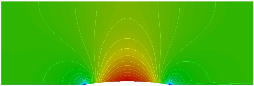
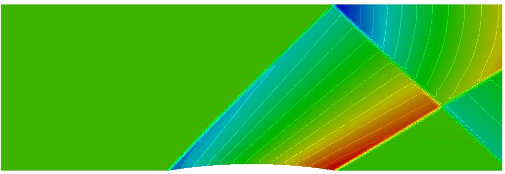
Fig. 9.4.1 Mach number contours for flow over a bump using the AUSM+ scheme: subsonic (top) and supersonic (bottom).

9.5. Standard Limiters: Barth-Jespersen (BJ) and Venkatakrishnan (V)

This section summarizes common slope limiters used to prevent spurious oscillations near discontinuities while maintaining second-order accuracy where possible.

For a face \(k\) between cells \(i\) and \(j\), the limited reconstructions are

(9.5.1)\[q_k^{+}=q_i+\phi_i\nabla q_i\cdot \Delta r_{ik},\]

(9.5.2)\[q_k^{-}=q_j+\phi_j\nabla q_j\cdot \Delta r_{jk}.\]

The BJ/V limiter factor is computed as

(9.5.3)\[\begin{split}\phi_i^{\mathrm{BJ/V}}= \min_{\text{overall }t\text{ values}} \begin{cases} f^{\mathrm{BJ/V}}\!\left(\dfrac{q_i^{\max}-q_i}{q_t-q_i}\right), & q_t-q_i>0,\\[10pt] f^{\mathrm{BJ/V}}\!\left(\dfrac{q_i^{\min}-q_i}{q_t-q_i}\right), & q_t-q_i<0,\\[10pt] 1, & q_t-q_i=0, \end{cases}\end{split}\]

where the BJ limiter uses

(9.5.4)\[f^{\mathrm{BJ}}\!\left(\frac{a}{b}\right)=\min\!\left(1,\frac{a}{b}\right),\]

and the Venkatakrishnan limiter uses

(9.5.5)\[f^{\mathrm{V}}\!\left(\frac{a}{b}\right) = \frac{1}{b} \left( \frac{(a^2+\epsilon^2)b+2b^2a}{a^2+2b^2+ab+\epsilon^2} \right).\]

with

(9.5.6)\[\epsilon^2=(K\Delta h)^3.\]

The cellwise bounds are

(9.5.7)\[q_i^{\max}=\max\!\left[q_i,\max_{j\in V(i)}(q_j)\right],\]

(9.5.8)\[q_i^{\min}=\min\!\left[q_i,\min_{j\in V(i)}(q_j)\right].\]

and the limiter enforces

(9.5.9)\[q_i^{\min}\le q_t\le q_i^{\max}.\]

The “test values” are defined as:

(9.5.10)\[q_t^{(v)}=q_i+\nabla q_i\cdot \Delta r_{il}, \qquad l\in v(i),\]

(9.5.11)\[q_t^{(f)}=q_i+\nabla q_i\cdot \Delta r_{ik}, \qquad \partial\Omega_k\subset \partial\Omega_i.\]

9.6. Multidimensional Limiting Process (MLP) Limiters

The multidimensional limiting process controls a reconstructed field using vertex-connected information rather than only face-neighbor values. The original unstructured MLP construction follows Park, Yoon, and Kim [PYK10]; MLP-PW introduces the pressure-weighted strict/weak blend of Zhang, Liu, and Chen [ZLC18].

Both methods use the piecewise-linear reconstruction introduced in Eqs. (9.5.1) and (9.5.2). For an arbitrary point \(\mathbf{x}\) in cell \(i\), write

(9.6.1)\[q_i^{L}(\mathbf{x}) =q_i+\psi_i\nabla q_i\cdot(\mathbf{x}-\mathbf{x}_i), \qquad 0\le\psi_i\le 1.\]

Stream uses the differentiable Venkatakrishnan response in Eq. (9.5.5) for both MLP variants. The difference between the methods is therefore the location at which the unlimited reconstruction is tested and the bounds supplied to that common response.

In the implementation, each local response is bounded below by zero and the cellwise minimum is initialized to one. A signed perturbation of magnitude \(10^{-30}\) regularizes the limiting \(0/0\) case. Consequently, both MLP variants preserve the admissible interval \(0\le\psi_i\le 1\).

Common MLP Assembly Pattern

1. Construct admissible upper and lower bounds from vertex-connected cell averages.

2. Evaluate the unlimited reconstruction increment at each MLP test location.

3. Apply the Venkatakrishnan response using the bound selected by the sign of that increment.

4. Take the minimum response over every test location in the cell.

The original MLP test locations are vertices. The MLP-PW test locations are face centers.

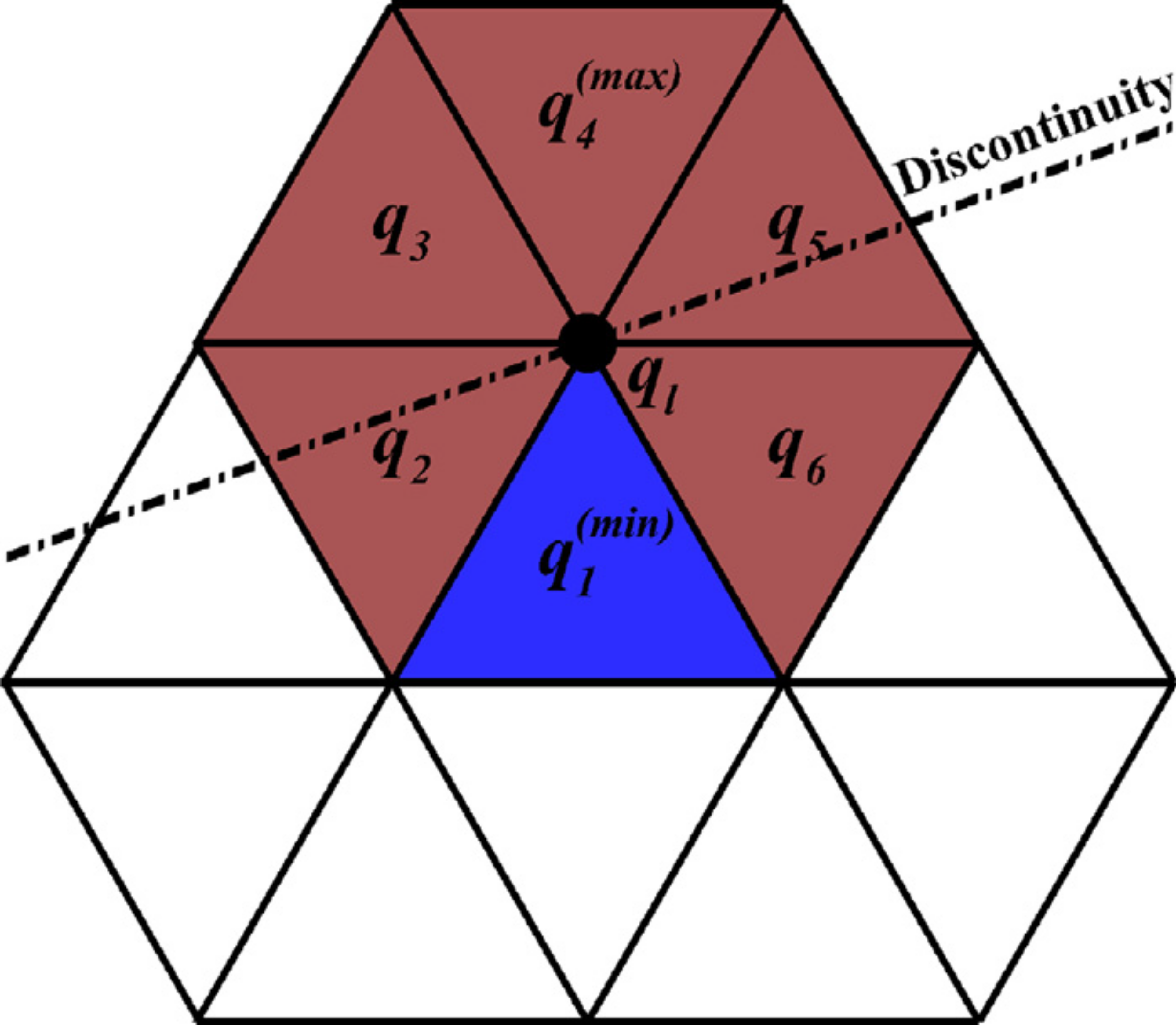
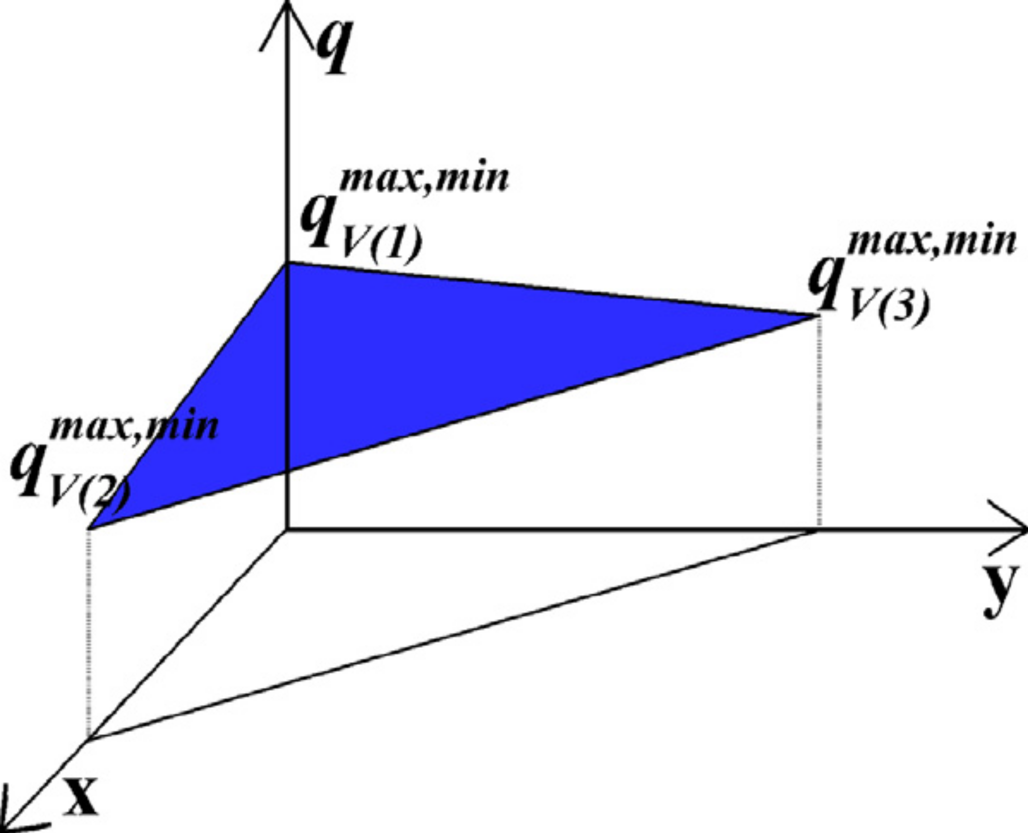
Fig. 9.6.1 Schematic diagrams of the unstructured MLP limiter.

9.6.1. Original Unstructured MLP Limiter

Let \(v(i)\) be the vertices of cell \(i\), and let \(V(l)\) be the cells sharing vertex \(l\). The admissible interval at that vertex is formed directly from the cell averages in \(V(l)\):

(9.6.1.1)\[q_{V(l)}^{\max}=\max_{j\in V(l)}q_j, \qquad q_{V(l)}^{\min}=\min_{j\in V(l)}q_j.\]

Because \(i\in V(l)\) for every vertex of cell \(i\), this interval always contains \(q_i\). The unlimited increment from the cell center to vertex \(l\) is

(9.6.1.2)\[\Delta^-_{il}=\nabla q_i\cdot\Delta\mathbf{r}_{il}, \qquad \Delta\mathbf{r}_{il}=\mathbf{x}_l-\mathbf{x}_i.\]

The original MLP coefficient is the minimum vertex response

(9.6.1.3)\[\begin{split}\psi_i^{\mathrm{MLP}} = \min_{l\in v(i)} \begin{cases} f_{\mathrm{V}}\!\left(q_{V(l)}^{\max}-q_i,\Delta^-_{il},\epsilon_i^2\right), & \Delta^-_{il}>0,\\[8pt] f_{\mathrm{V}}\!\left(q_{V(l)}^{\min}-q_i,\Delta^-_{il},\epsilon_i^2\right), & \Delta^-_{il}<0,\\[8pt] 1, & \Delta^-_{il}=0. \end{cases}\end{split}\]

Here \(f_{\mathrm{V}}(\Delta^+,\Delta^-,\epsilon^2)\) denotes the Venkatakrishnan response of Eq. (9.5.5), with \(a=\Delta^+\) and \(b=\Delta^-\). The same coefficient multiplies the cell gradient for every face reconstruction from cell \(i\).

Original MLP Stencil

The extrema at a vertex use the cell averages of every cell sharing that vertex. Physical-boundary vertices remain part of the cell’s test set, but a boundary-face state is not inserted into the vertex extrema.

9.6.2. Unstructured MLP-PW Limiter

MLP-PW blends two different admissible envelopes. The weak envelope is constructed independently at each face from the extrema of the cell averages that share its vertices. The strict envelope is constructed once for the cell from inverse-distance averages at all of its vertices.

MLP-PW Bound Roles

• Weak side: face-local bounds; less restrictive away from shocks.

• Strict side: cell-wide bounds from averaged vertex values; more restrictive near shocks.

• Pressure weight: blends weak and strict bounds before the local limiter response is evaluated.

For face \(k\), the weak bounds are

(9.6.2.1)\[q_{k,\mathrm{w}}^{\max}=\frac{\sum_{l\in v(k)}q_{V(l)}^{\max}}{n_{v(k)}}, \qquad q_{k,\mathrm{w}}^{\min}=\frac{\sum_{l\in v(k)}q_{V(l)}^{\min}}{n_{v(k)}}.\]

The corresponding weak-MLP condition applies to the reconstructed value on each side of that face:

(9.6.2.2)\[q_{k,\mathrm{w}}^{\min}\le q_k^{\pm}\le q_{k,\mathrm{w}}^{\max}.\]

For the strict envelope, first compute an averaged value at vertex \(l\):

(9.6.2.3)\[\bar{q}_l=\frac{\sum_{j\in V(l)}\omega_{lj}q_j}{\sum_{j\in V(l)}\omega_{lj}}, \qquad \omega_{lj}\ge 0.\]

The inverse-distance weights used here are

(9.6.2.4)\[\omega_{lj}=\frac{1}{\left|\Delta r_{lj}\right|}.\]

The accumulated weight in the denominator of Eq. (9.6.2.3) is regularized by a \(10^{-20}\) perturbation in the implementation.

The raw strict bounds are the extrema of those averaged vertex values over cell \(i\):

(9.6.2.5)\[q_{i,\mathrm{s}}^{\max}=\max_{l\in v(i)}\left(\bar{q}_l\right), \qquad q_{i,\mathrm{s}}^{\min}=\min_{l\in v(i)}\left(\bar{q}_l\right).\]

At a discrete local extremum, every averaged vertex value can lie on the same side of \(q_i\). In that case the raw strict interval does not contain the cell average, so no nonnegative conservative slope coefficient can enforce it. Stream therefore uses the feasible strict envelope

(9.6.2.6)\[\widetilde q_{i,\mathrm{s}}^{\max}=\max\!\left(q_i,q_{i,\mathrm{s}}^{\max}\right), \qquad \widetilde q_{i,\mathrm{s}}^{\min}=\min\!\left(q_i,q_{i,\mathrm{s}}^{\min}\right).\]

9.6.2.1. Pressure Weight Function

The pressure sensor continues to use the raw strict pressure extrema from Eq. (9.6.2.5):

(9.6.2.7)\[\omega_p=\left(\frac{p_{i,\mathrm{s}}^{\min}}{p_{i,\mathrm{s}}^{\max}}\right)^3.\]

For positive absolute pressure, \(0\le\omega_p\le 1\). Thus \(\omega_p\rightarrow 0\) selects the strict side near a strong pressure variation, while \(\omega_p\rightarrow 1\) selects the weak side in smoother regions. Stream also provides the two endpoints of the blend:

(9.6.2.8)\[\begin{split}\omega_p^{\mathrm{impl}}= \begin{cases} \left(p_{i,\mathrm{s}}^{\min}/p_{i,\mathrm{s}}^{\max}\right)^3, & m=0,\quad\text{pressure weighted},\\[4pt] 0, & m=1,\quad\text{strict},\\[4pt] 1, & m=2,\quad\text{weak}. \end{cases}\end{split}\]

The implementation fact mlp_modes selects \(m\) and defaults to the pressure-weighted mode. It affects MLP-PW only; the original MLP construction has no strict/weak blend. The unlimited increment from cell \(i\) to face \(k\) is

(9.6.2.9)\[\Delta^-_{ik}=\nabla q_i\cdot\Delta\mathbf{r}_{ik}, \qquad \Delta\mathbf{r}_{ik}=\mathbf{x}_k-\mathbf{x}_i.\]

The MLP-PW coefficient is the minimum response over all faces of the cell, including physical boundary faces:

(9.6.2.10)\[\begin{split}\psi_i^{\mathrm{MLP\text{-}pw}} = \min_{k\in\mathcal{F}(i)} \begin{cases} f_{\mathrm{V}}\!\left(\omega_p q_{k,\mathrm{w}}^{\max}+(1-\omega_p)\widetilde q_{i,\mathrm{s}}^{\max}-q_i,\Delta^-_{ik},\epsilon_i^2\right), & \Delta^-_{ik}>0,\\[8pt] f_{\mathrm{V}}\!\left(\omega_p q_{k,\mathrm{w}}^{\min}+(1-\omega_p)\widetilde q_{i,\mathrm{s}}^{\min}-q_i,\Delta^-_{ik},\epsilon_i^2\right), & \Delta^-_{ik}<0,\\[8pt] 1, & \Delta^-_{ik}=0. \end{cases}\end{split}\]

Each local response is restricted to be nonnegative, and the facewise minimum begins from unity. The final reconstruction coefficient therefore satisfies \(0\le\psi_i^{\mathrm{MLP\text{-}pw}}\le 1\). A coefficient of zero recovers the cell average and cannot reverse the unlimited gradient.

9.6.3. Stream Response Scaling and Rule Behavior

The paper form in Eq. (9.5.6) describes the role of the Venkatakrishnan smoothing parameter. Stream evaluates that parameter using a cell-volume scale and a local reference magnitude. Let \(\Omega_i\) be the cell volume, let \(\Omega_g=\sum_i\Omega_i\) be the total grid volume, let \(\mathcal{F}_{\mathrm{int}}(i)\) and \(\mathcal{F}_b(i)\) be the interior and physical-boundary faces of the cell, and let \(n(k)\) be the neighboring cell across interior face \(k\). With \(N_i^{\mathrm{ref}}=1+|\mathcal{F}_{\mathrm{int}}(i)|+|\mathcal{F}_b(i)|\), the scalar reference magnitude is

(9.6.3.1)\[q_i^{\mathrm{ref}} =\delta_q+\frac{1}{N_i^{\mathrm{ref}}} \left[ q_i^2 +\sum_{k\in\mathcal{F}_{\mathrm{int}}(i)}q_{n(k)}^2 +\sum_{k\in\mathcal{F}_b(i)}q_{k,b}^2 \right]^{1/2}, \qquad \delta_q=10^{-20}.\]

The scalar smoothing parameter is

(9.6.3.2)\[\epsilon_i^2 =\frac{6K_{\ell}^{3}}{\pi\Omega_g}\, \Omega_i\left(q_i^{\mathrm{ref}}\right)^2.\]

This scaling is used by both original MLP and MLP-PW. The symbol \(K_{\ell}\) corresponds to the Stream input parameter Kl. Increasing \(K_{\ell}\) increases the smooth-region tolerance of the Venkatakrishnan response.

For a three-component vector field, the vertex extrema, strict and weak bounds, increments, and limiter responses are evaluated component by component. Stream first computes a scalar reference \(q_{i,\alpha}^{\mathrm{ref}}\) for each Cartesian component and then uses

(9.6.3.3)\[q_{i,v}^{\mathrm{ref}} =\left[ \left(q_{i,x}^{\mathrm{ref}}\right)^2 +\left(q_{i,y}^{\mathrm{ref}}\right)^2 +\left(q_{i,z}^{\mathrm{ref}}\right)^2 \right]^{1/2}\]

in Eq. (9.6.3.2). Thus all three vector components use the same smoothing parameter even though their bounds and final limiter coefficients remain componentwise.

Stream Implementation Summary

• Original MLP: test the reconstruction at every vertex of the cell and take the minimum vertex response.

• MLP-PW: test the reconstruction at every interior and physical-boundary face center and take the minimum face response.

• Nodal data: construct extrema and inverse-distance averages from the cell averages sharing each vertex; boundary-face states do not replace those nodal values.

• Pressure sensor: compute \(\omega_p\) from the raw averaged-vertex pressure extrema, while the limiter numerator uses the feasible strict envelope of Eq. (9.6.2.6).

• Scalar and three-component vector fields: apply the same construction to scalars and to each vector component, with the shared vector smoothing scale described above.

• Forced first order: set every resulting scalar or vector limiter coefficient to zero in a cell selected for first-order reconstruction.

The implementation mapping is summarized below. These names identify the corresponding Loci facts; they do not replace the theory notation used in the derivation.

Mathematical role	Stream implementation quantity
Vertex extrema \(q_{V(l)}^{\max,\min}\)	NodalMax(X), NodalMin(X)
Inverse-distance vertex average \(\bar q_l\)	Cell2Node(X)
Weak face bounds \(q_{k,\mathrm{w}}^{\max,\min}\)	FaceNodalAverage(NodalMax/Min(X))
Raw strict bounds \(q_{i,\mathrm{s}}^{\max,\min}\)	CellNodalMax/Min(Cell2Node(X))
Pressure weight \(\omega_p\)	MLPWeightingFactor
Scalar coefficient \(\psi_i\)	streamlimiters::limiters(X)
Three-component vector coefficient \(\boldsymbol{\psi}_i\)	streamlimiters::limiterv3d(X)

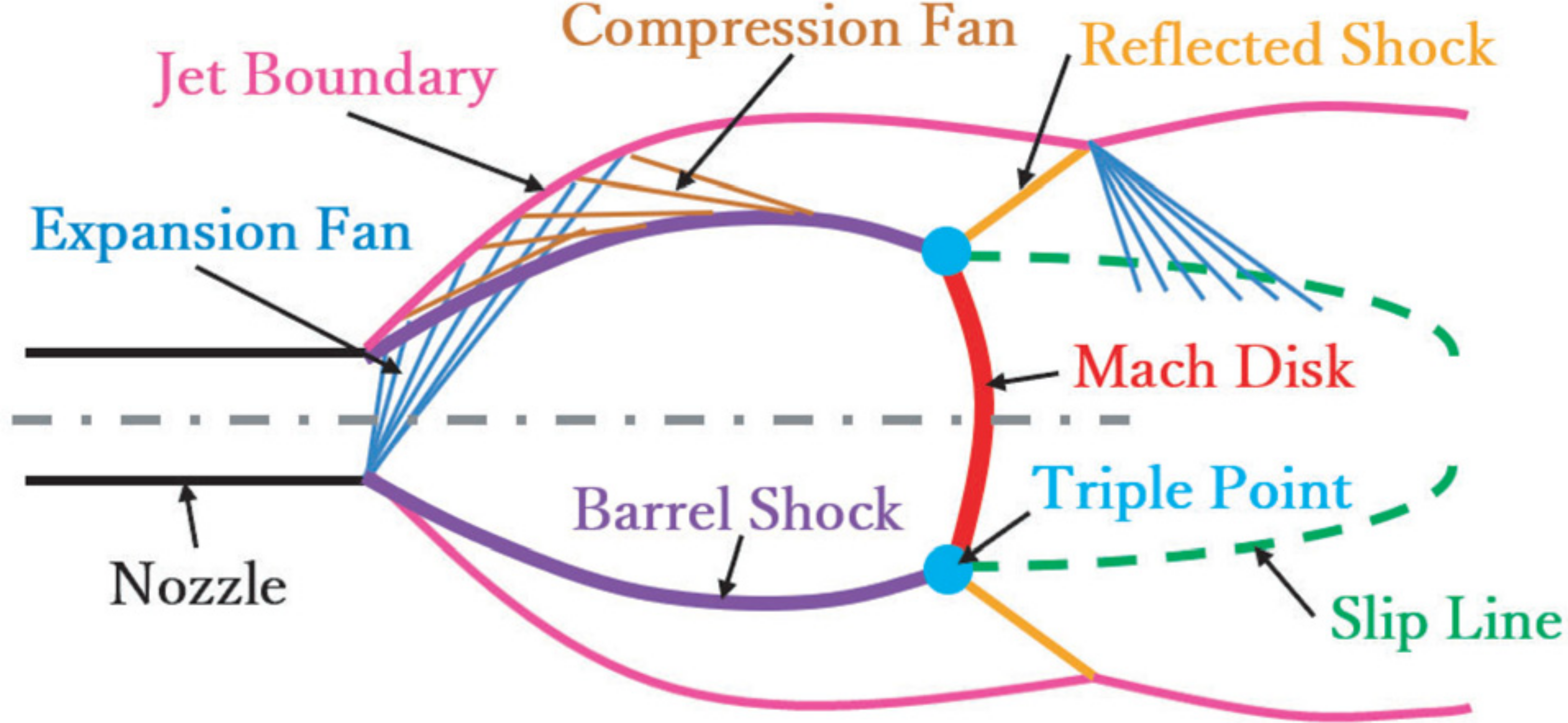
Fig. 9.6.3.1 Key flow features including Mach disk in an under-expanded jet.

9.7. Blended Hybrid SLAU/SLAU2 Dissipation Framework

The hybrid SLAU/SLAU2 method is a blended scalar-dissipation correction. It modifies the momentum dissipation level while preserving the base SLAU/SLAU2 flux structure. It does not replace the SLAU-family numerical flux with a full HLLE-family Riemann flux. Instead, each optional backend supplies an effective mass-dissipation magnitude that is blended with the baseline SLAU/SLAU2 dissipation. The objective is to retain low dissipation in smooth/all-speed regions and introduce stronger dissipation near strong shocks to improve robustness (including carbuncle resistance).

For each face, define the baseline SLAU dissipation magnitude:

(9.7.1)\[\Delta m_f^{\mathrm{SLAU}} = \left|\rho_f\left(V_f-V_{g,f}\right)\right|,\]

where \(\rho_f\) is face density, \(V_f\) is face volumetric flux, and \(V_{g,f}\) is grid volumetric flux.

Define a pressure-ratio weight at each cell:

(9.7.2)\[\omega_{p,i} = \left(\frac{p_{v(i)}^{\min}}{p_{v(i)}^{\max}}\right)^3, \qquad 0\le \omega_{p,i}\le 1,\]

and take the face value

(9.7.3)\[\omega_{p,f}=\min\!\left(\omega_{p,L},\omega_{p,R}\right).\]

The hybrid dissipation magnitude is blended as

(9.7.4)\[\Delta m_f^{\mathrm{hyb}} = \left(1-\omega_{p,f}\right)\Delta m_f^{B} +\omega_{p,f}\Delta m_f^{\mathrm{SLAU}},\]

where \(\Delta m_f^{B}\) is the backend dissipation model.

The correction added to the momentum equation is

(9.7.5)\[\mathbf{S}_f^{\mathrm{hyb}} = \frac{1}{2}\left(\Delta m_f^{\mathrm{hyb}}-\Delta m_f^{\mathrm{SLAU}}\right) \left(\mathbf{u}_L-\mathbf{u}_R\right).\]

This source is assembled antisymmetrically:

(9.7.6)\[\mathbf{R}_{\rho\mathbf{u},L}\leftarrow \mathbf{R}_{\rho\mathbf{u},L}-\mathbf{S}_f^{\mathrm{hyb}}, \qquad \mathbf{R}_{\rho\mathbf{u},R}\leftarrow \mathbf{R}_{\rho\mathbf{u},R}+\mathbf{S}_f^{\mathrm{hyb}}.\]

From Eq. (9.7.4), two useful limits follow:

• \(\omega_{p,f}\to 1\): \(\Delta m_f^{\mathrm{hyb}}\to\Delta m_f^{\mathrm{SLAU}}\) (hybrid correction vanishes).

• \(\omega_{p,f}\to 0\): \(\Delta m_f^{\mathrm{hyb}}\to\Delta m_f^{B}\) (full backend dissipation).

9.7.1. Backend Scalar Dissipation Models

9.7.1.1. 1. van Leer/Hanel backend

Define

(9.7.1.1)\[M_L=\frac{u_{nL}}{c_L},\qquad M_R=\frac{u_{nR}}{c_R},\]

with split Mach functions

(9.7.1.2)\[\begin{split}M_L^{+}= \begin{cases} \frac{1}{4}(M_L+1)^2,& |M_L|<1,\\[4pt] \frac{1}{2}(M_L+|M_L|),& |M_L|\ge 1, \end{cases} \qquad M_R^{-}= \begin{cases} -\frac{1}{4}(M_R-1)^2,& |M_R|<1,\\[4pt] \frac{1}{2}(M_R-|M_R|),& |M_R|\ge 1. \end{cases}\end{split}\]

Then

(9.7.1.3)\[\Delta m_f^{\mathrm{VL}} = \left|\rho_L c_L M_L^{+}-\rho_R c_R M_R^{-}\right|A_f.\]

9.7.1.2. 2. HLLE-family-inspired backend primitives

For the HLLE-family-inspired scalar backends (HLLE, HLLEM, LM-HLLEM, and HLLEMCC), define

(9.7.1.4)\[u_{nL}=\mathbf{u}_L\cdot \mathbf{n},\quad u_{nR}=\mathbf{u}_R\cdot \mathbf{n},\quad \bar{c}=\max\!\left(\frac{c_L+c_R}{2},\varepsilon_c\right),\quad \bar{\rho}=\max\!\left(\frac{\rho_L+\rho_R}{2},\varepsilon_\rho\right),\]

(9.7.1.5)\[S_L=\min\!\left(u_{nL}-c_L,\,u_{nR}-c_R\right),\qquad S_R=\max\!\left(u_{nL}+c_L,\,u_{nR}+c_R\right),\]

and the jump scale

(9.7.1.6)\[J_f= \max\!\left( \left|\rho_R-\rho_L\right| +\bar{\rho}\frac{|u_{nR}-u_{nL}|}{\bar{c}} +\frac{|p_R-p_L|}{\bar{c}^2}, \;\varepsilon_J \right),\]

where \(\varepsilon_c\) and \(\varepsilon_\rho\) are small internal positive floors, and \(\varepsilon_J\) is a positive floor on the combined state-jump measure.

The HLLE-inspired backend dissipation magnitude is

(9.7.1.7)\[\Delta m_f^{\mathrm{HLLE}} = \frac{1}{2}|S_R-S_L|\,J_f\,A_f.\]

9.7.1.3. 3. HLLEM-inspired backend

Define shock/contact sensors:

(9.7.1.8)\[\psi_s=\min\!\left(1,\frac{|p_R-p_L|}{\max\!\left(\frac{|p_L|+|p_R|}{2},\,p_{\mathrm{ref}}\right)}\right), \qquad \psi_c=1-\psi_s,\]

where \(p_{\mathrm{ref}}\) is a positive pressure-normalization floor used by the shock sensor.

then reduce the HLLE-inspired backend dissipation in contact/shear-dominated regions:

(9.7.1.9)\[r_c=0.6\,\mathrm{clip}(C_{\mathrm{contact}},0,1)\,\psi_c, \qquad \Delta m_f^{\mathrm{HLLEM}}=(1-r_c)\Delta m_f^{\mathrm{HLLE}}.\]

9.7.1.4. 4. LM-HLLEM-inspired backend

Define a face Mach number and bounds:

(9.7.1.10)\[M_f=\frac{\left|\frac{u_{nL}+u_{nR}}{2}\right|}{\bar{c}}, \quad M_{\min}=\mathrm{clip}(M_{\mathrm{floor}},10^{-6},1), \quad M_{\max}=\max(M_{\min},M_{\mathrm{ceiling}}),\]

then apply low-Mach scaling:

(9.7.1.11)\[f_{\mathrm{LM}}=\min\!\left(1,\max\!\left(M_{\min},\frac{M_f}{M_{\max}}\right)\right), \qquad \Delta m_f^{\mathrm{LM\text{-}HLLEM}}=f_{\mathrm{LM}}\Delta m_f^{\mathrm{HLLEM}}.\]

9.7.1.5. 5. HLLEMCC-inspired backend

The HLLEMCC-inspired backend restores dissipation toward the HLLE-inspired backend in strong-shock regions:

(9.7.1.12)\[c_c=\min\!\left(1,\mathrm{clip}(C_{\mathrm{carbuncle}},0,1)\,\psi_s\right), \qquad \Delta m_f^{\mathrm{HLLEMCC}} = \Delta m_f^{\mathrm{HLLEM}} +c_c\left(\Delta m_f^{\mathrm{HLLE}}-\Delta m_f^{\mathrm{HLLEM}}\right).\]

9.7.2. Conceptual Summary

• van Leer/Hanel provides the legacy split-flux dissipation reference.

• HLLE-inspired backend dissipation provides the strongest baseline backend in strong-shock regimes.

• HLLEM-inspired backend dissipation reduces HLLE-like dissipation where shocks are weak to better preserve contact/shear features.

• LM-HLLEM-inspired backend dissipation further reduces excessive dissipation in low-Mach regions.

• HLLEMCC-inspired backend dissipation increases robustness by recovering HLLE-like dissipation as shock strength grows.

These backend names identify scalar dissipation models used inside the blended hybrid SLAU/SLAU2 correction. They should not be read as standalone replacement flux functions for the full conservative state vector.

9.8. References

[PYK10]

J.S. Park, S.H. Yoon, and C. Kim. Multi-dimensional limiting process for hyperbolic conservation laws on unstructured grids. Journal of Computational Physics, 229(3):788–812, 2010.

[ZLC18]

F. Zhang, J. Liu, and B. Chen. Modified multi-dimensional limiting process with enhanced shock stability on unstructured grids. Computers and Fluids, 161:171–188, 2018.