16. Pressure-Temperature-Equilibrium Multi-Material Algebraic-VOF Framework#

This chapter describes a pressure-temperature-equilibrium (PTE) model for compressible flow with immiscible materials. All materials present in a cell share one pressure, temperature, and velocity. Each material has its own equation of state (EOS) and composition. Species mix and diffuse within a material. Finite-rate chemistry and transfer between materials enter through conservative sources. Common pressure and temperature do not imply chemical or phase equilibrium.

The model advances every species density, mixture momentum, and mixture energy, using total enthalpy as the energy-equation unknown. Material and mixture mass balances follow by summing the species balances. Material volume fractions are obtained from the transported masses and EOS densities. Pressure correction enforces the requirement that the material volumes fill the cell.

The finite-volume discretization uses a fixed mesh, the first-order backward differentiation formula (BDF1), algebraic volume-of-fluid (VOF) reconstruction, and a segregated pressure-based iteration.

16.1. Materials and Species#

Let $m=1,\ldots,N_m$ index materials and $s=1,\ldots,N_s$ index species. The set $\mathcal K_m$ contains the species indices belonging to material $m$. These sets are disjoint and together contain all species indices. The same chemical constituent can be represented separately in two materials, such as a liquid and its vapor.

For a cell of volume $\Omega$, the volume fraction $\alpha_m$ is the fraction occupied by material $m$. An admissible state satisfies

(16.1.1)#\[0\le\alpha_m\le1 \qquad \sum_{m=1}^{N_m}\alpha_m=1\]

The transported species density $z_{ms}$ is the mass of species $s$ in material $m$ per unit cell volume. Its sum within a material gives the material mass density

(16.1.2)#\[q_m=\sum_{s\in\mathcal K_m}z_{ms}\]

The mixture density is $\rho=\sum_m q_m$. Both $z_{ms}$ and $q_m$ are mass per unit mixture volume. For a present material, the EOS gives its intrinsic density $\rho_m$, measured per unit volume occupied by that material. Thus

(16.1.3)#\[q_m=\alpha_m\rho_m\]

The volume fraction is recovered as $\alpha_m=q_m/\rho_m$. The species mass fraction within a present material is

(16.1.4)#\[\widetilde Y_s^{(m)}=\frac{z_{ms}}{q_m} \qquad q_m>0\]

The vector $\widetilde{\vec Y}^{(m)}$ is the composition supplied to that material’s EOS. Its components satisfy

(16.1.5)#\[\widetilde Y_s^{(m)}\ge0 \qquad \sum_{s\in\mathcal K_m}\widetilde Y_s^{(m)}=1\]

For a one-species material, $\widetilde Y_s^{(m)}=1$ and $z_{ms}=q_m$. Its species balance is still solved. When a material is absent, $q_m=0$, all its species densities and its volume fraction are zero, and its composition and EOS state are undefined. Mixture sums involving material properties include only present materials.

The mass fraction of material $m$ in the mixture is

(16.1.6)#\[w_m=\frac{q_m}{\rho} \qquad \sum_{m=1}^{N_m}w_m=1\]

For $s\in\mathcal K_m$ in a present material, the mixture species mass fraction is

(16.1.7)#\[Y_s=\frac{z_{ms}}{\rho}=w_m\widetilde Y_s^{(m)}\]

An absent material has $w_m=0$ and $Y_s=0$ for its species. The mixture species fractions are nonnegative and satisfy

(16.1.8)#\[\sum_{s\in\mathcal K_m}Y_s=w_m \qquad \sum_{s=1}^{N_s}Y_s=1\]

These fractions describe species amounts in the whole mixture. Material thermodynamics and species diffusion use the composition within each material.

16.2. Solved and Derived Variables#

The conserved quantities and the unknowns used in the segregated solves are listed below. Here $E$ and $h_t$ denote mixture specific total energy and total enthalpy, respectively.

Equation	Conserved quantity	Solved variable
Material species	$z_{ms}$	Species density $z_{ms}$
Momentum	$\rho\vec u$	Velocity $\vec u$
Total energy	$\rho E=\rho h_t-p$	Total enthalpy $h_t$

Species sums give the material mass densities $q_m$ and mixture density $\rho$. Composition and mass fractions follow from these densities as defined in Materials and Species. At the common pressure and temperature, each present material’s EOS supplies its intrinsic density $\rho_m$, enthalpy, and other thermodynamic properties. Its volume fraction is then $\alpha_m=q_m/\rho_m$.

At fixed pressure, temperature is obtained by matching the mixture enthalpy to the solved total enthalpy minus kinetic energy. Pressure correction enforces that the material volumes fill the cell and corrects the velocity and face volume flux. Transport, pressure, and temperature are coupled by the iteration in Segregated Nonlinear Algorithm.

16.2.1. Material appearance#

Transport or a physical source can introduce material into a cell where it was absent. The resulting species densities determine its mass and composition, and its EOS density determines its volume fraction. A source must supply consistent species, momentum, and energy contributions; its material mass source is the sum of its species sources, as required by Eq. (16.5.1.5). Face transport into cells with absent materials is described in Material-Appearance Face Reference.

16.3. Thermodynamic Definitions#

Material thermodynamic properties are evaluated from pressure, temperature, and material composition. The materials share the same cell pressure and temperature, but each material EOS receives only its own composition.

It is useful to distinguish a material constitutive model from an evaluated material state. Let $\mathcal{E}_m$ denote the EOS mapping for material $m$. A cell-local thermodynamic state is the result of evaluating that mapping:

(16.3.1)#\[\mathbf{s}_m(\mathbf{x},t) = \mathcal{E}_m\!\left( p(\mathbf{x},t), T(\mathbf{x},t), \widetilde{\vec{Y}}^{(m)}(\mathbf{x},t) \right).\]

For every active material, the state $\mathbf{s}_m$ supplies finite $\rho_m>0$, $h_m$, $e_m$, the partial specific enthalpies required by species diffusion and phase transfer, the physical sound speed $c_m$ at fixed material composition, and the thermodynamic derivatives required by the PTE closure. It also reports whether the state lies on the material’s assigned phase branch and inside its valid thermodynamic domain. The constitutive state is determined only by the local $(p,T,\widetilde{\vec{Y}}^{(m)})$ and the material model $\mathcal E_m$.

The evaluated state supplies the intrinsic material density and static thermodynamic enthalpy:

(16.3.2)#\[\rho_m = \rho_m\!\left( p,T,\widetilde{\vec{Y}}^{(m)};\mathcal{E}_m \right),\]

(16.3.3)#\[h_m = h_m\!\left( p,T,\widetilde{\vec{Y}}^{(m)};\mathcal{E}_m \right).\]

It also supplies the fixed-composition derivatives

(16.3.4)#\[\rho_{m,p} = \left(\frac{\partial\rho_m}{\partial p}\right)_{T,\widetilde{\vec{Y}}^{(m)}}, \qquad \rho_{m,T} = \left(\frac{\partial\rho_m}{\partial T}\right)_{p,\widetilde{\vec{Y}}^{(m)}}, \qquad h_{m,p} = \left(\frac{\partial h_m}{\partial p}\right)_{T,\widetilde{\vec{Y}}^{(m)}}, \qquad h_{m,T} = \left(\frac{\partial h_m}{\partial T}\right)_{p,\widetilde{\vec{Y}}^{(m)}}.\]

The mapping $\mathcal E_m$ returns these derivatives with $\rho_m$ and $h_m$, evaluated at the same $(p,T,\widetilde{\vec{Y}}^{(m)})$ on the assigned EOS branch.

For the species-diffusion energy flux, let $M_m=q_m\Omega$ be the material mass in the cell and $M_s=z_{ms}\Omega$ the mass of species $s\in\mathcal K_m$. The extensive material enthalpy is $H_m=M_mh_m$. The same evaluated state supplies the partial specific enthalpy

(16.3.5)#\[\bar h_{ms} = \left( \frac{\partial H_m}{\partial M_s} \right)_{p,T,M_{\ell\ne s},\,\ell\in\mathcal K_m} \qquad s\in\mathcal{K}_m.\]

Extensivity gives

(16.3.6)#\[H_m = \sum_{s\in\mathcal K_m}M_s\bar h_{ms}, \qquad h_m = \sum_{s\in\mathcal K_m}\widetilde Y_s^{(m)}\bar h_{ms}.\]

The partial specific enthalpy is evaluated at the complete material composition with the same reference convention as $h_m$. The effect of consistent enthalpy-reference shifts is derived in Enthalpy references.

Each $\mathcal E_m$ defines the mixing rule for the species inside material $m$. There is no cross-material EOS and no second reconstruction of a material state from mixture species fractions. The mixture volume is the sum of the independently evaluated material volumes:

(16.3.7)#\[\Omega=\sum_m\frac{M_m}{\rho_m}, \qquad \alpha_m=\frac{q_m}{\rho_m}, \qquad \sum_m\frac{q_m}{\rho_m}=1.\]

The material internal energy is related to its static enthalpy by

(16.3.8)#\[e_m=h_m-\frac{p}{\rho_m}.\]

The mixture level is the level of the common pressure, velocity, and temperature fields. Each material nevertheless retains its own evaluated EOS state. The mixture density is mass per mixture volume, so each material contributes according to the volume fraction it occupies:

(16.3.9)#\[\rho=\sum_{m=1}^{N_m}q_m=\sum_{m=1}^{N_m}\alpha_m\rho_m\]

The mixture static thermodynamic enthalpy is a specific quantity per unit mixture mass, so it is averaged with the material mass fractions:

(16.3.10)#\[h=\sum_{m=1}^{N_m}\frac{\alpha_m \rho_m}{\rho} h_m = \sum_{m=1}^{N_m} w_m h_m\]

The mixture internal-energy density follows from the same material masses:

(16.3.11)#\[\rho e = \sum_{m=1}^{N_m}\alpha_m\rho_m e_m = \rho h-p,\]

where the final equality uses $\sum_m\alpha_m=1$. Defining $K=\frac12\lVert\vec{u}\rVert^2$, the mixture total energy is

(16.3.12)#\[E=e+K, \qquad \rho h_t-p=\rho E.\]

The total enthalpy is defined as the static thermodynamic enthalpy plus kinetic energy:

(16.3.13)#\[h_t=h+\frac{1}{2}\lVert\vec{u}\rVert^2\]

16.3.1. Pressure-temperature compatibility#

At a fixed transported state, the species densities $z_{ms}$, their material sums $q_m$, velocity $\vec{u}$, and total enthalpy $h_t$ are known. The materials present in the cell form the set

(16.3.1.1)#\[\mathcal A=\{m:q_m>0\}\]

For each $m\in\mathcal A$, the species densities determine $\widetilde{\vec{Y}}^{(m)}$ through Eq. (16.1.4). The material EOS branches are also held fixed. The common pressure and temperature must satisfy the volume and enthalpy compatibility conditions below.

With the kinetic energy defined above, the mixture density and target static enthalpy are

(16.3.1.2)#\[\rho=\sum_{m\in\mathcal A}q_m, \qquad h^{\mathrm{tar}}=h_t-K.\]

A trial $(p,T)$ supplies $\rho_m(p,T,\widetilde{\vec{Y}}^{(m)})$ and $h_m(p,T,\widetilde{\vec{Y}}^{(m)})$ from each active material EOS. Because $q_m\Omega$ is the material mass in a cell, $q_m/\rho_m$ is the fraction of the cell volume occupied by that material. Additive volume requires these fractions to sum to one. Equation (16.3.10) also requires $\sum_{m\in\mathcal A}q_mh_m=\rho h^{\mathrm{tar}}$. These two requirements define the closure residuals

(16.3.1.3)#\[F_V(p,T) = \sum_{m\in\mathcal A} \frac{q_m}{\rho_m(p,T,\widetilde{\vec{Y}}^{(m)})}-1 = \sum_{m\in\mathcal A}\alpha_m(p,T)-1 =0, \qquad F_H(p,T) = \sum_{m\in\mathcal A}q_m \left[ h_m(p,T,\widetilde{\vec{Y}}^{(m)})-h^{\mathrm{tar}} \right] =0.\]

Here $\alpha_m(p,T)=q_m/\rho_m(p,T,\widetilde{\vec{Y}}^{(m)})$ is a trial EOS-derived volume fraction, not an independent input. The residual $F_V$ is dimensionless. The residual $F_H$ has units $\mathrm{J/m^3}$, equivalently $\mathrm{Pa}$; dividing it by $\rho$ gives the corresponding specific-enthalpy residual in $\mathrm{J/kg}$. These are compatibility conditions on the transported state, not additional conservation equations.

The same residuals enforce the total-energy representation. Using $e_m=h_m-p/\rho_m$ gives

(16.3.1.4)#\[\left(\sum_{m\in\mathcal A}q_m e_m+\rho K\right) -\left(\rho h_t-p\right) = F_H-pF_V.\]

Therefore, $F_V=F_H=0$ makes the total-energy density reconstructed from the material EOS states equal to the transported total-energy density while the material volumes fill the cell. At the coupled root, this enthalpy form is equivalent to the specific-volume and internal-energy PTE closure discussed in References [5] and [6].

Assume every active EOS branch is continuous over the common admissible interval and satisfies $c_{p,m}>0$ and $\rho_{m,p}>0$ there. Then

(16.3.1.5)#\[\left(\frac{\partial F_H}{\partial T}\right)_p = \sum_{m\in\mathcal A}q_m c_{p,m}>0, \qquad \left(\frac{\partial F_V}{\partial p}\right)_T = -\sum_{m\in\mathcal A} \frac{q_m\rho_{m,p}}{\rho_m^2} <0.\]

Thus, at fixed pressure, the enthalpy residual has at most one temperature root. A root exists in the selected interval when the active EOS temperature domains overlap and the endpoint residuals bracket zero. Both residuals generally depend on both $p$ and $T$.

For a fixed pressure $p$, the common-temperature inversion is the scalar problem

(16.3.1.6)#\[f_H(\theta) \equiv \frac{1}{\rho} \sum_{m\in\mathcal A}q_m \left[ h_m(p,\theta,\widetilde{\vec{Y}}^{(m)})-h^{\mathrm{tar}} \right], \qquad f_H(T)=0.\]

During this local solve, $p$, $q_m$, $z_{ms}$, $h^{\mathrm{tar}}$, the active set, and the material EOS branches remain fixed. Each active material EOS is evaluated at every trial temperature $\theta$.

CMIM uses this inversion both before and after pressure correction. The pre-pressure evaluation supplies the material densities and derivatives in Eq. (16.7.1.3). The pressure equation uses the local derivative of $F_V$ along $F_H=0$ together with the pressure-induced face-volume-flux response; it is not a local two-variable closure solve. After pressure correction, the corrected velocity defines $h^{\mathrm{tar}}$, the scalar inversion supplies the common temperature, and the material EOS states are evaluated at the corrected $(p,T)$. The complete stage order is given in Segregated Nonlinear Algorithm.

16.3.2. Initial state#

Prescribe the volume fractions, each present material’s composition, and the common pressure, temperature, and velocity. Fractions must satisfy Eqs. (16.1.1) and (16.1.5). The common pressure and temperature must lie within every present material’s EOS domain on its assigned branch.

Evaluate the present material densities and enthalpies, then initialize

(16.3.2.1)#\[z_{ms}=\alpha_m\rho_m\widetilde Y_s^{(m)} \qquad h_t=\sum_{m\in\mathcal A}\frac{q_m}{\rho}h_m +\frac12\lVert\vec u\rVert^2\]

Here $q_m$ and $\rho$ are the species sums. For an absent material, set its species densities to zero without evaluating its composition or EOS state; see Material appearance. These constructions give compatible mass, volume, and energy states, with $\rho h_t-p=\rho E$.

Thermodynamic compatibility does not imply mechanical balance. A field intended to remain at rest must also balance pressure against gravity and capillary forces; the conditions are given in Equilibria.

16.4. Mixture Viscosity and Heat Conduction#

For each material with positive partial density $q_m$, its transport model supplies the dynamic viscosity $\mu_m$ and thermal conductivity $\lambda_m$ at the common cell pressure and temperature and the material-local composition. The cell mixture properties are the normalized volume-fraction averages

(16.4.1)#\[\alpha_\Sigma=\sum_m\alpha_m, \qquad \mu_{\mathrm{mix}}=\frac{1}{\alpha_\Sigma}\sum_m\alpha_m\mu_m, \qquad \lambda_{\mathrm{mix}}=\frac{1}{\alpha_\Sigma}\sum_m\alpha_m\lambda_m.\]

An absent material has $\alpha_m=0$ and does not contribute. At closure, $\alpha_\Sigma=1$; the normalized form is retained during the nonlinear iteration when the volume-fraction sum may differ from unity.

For turbulent flow, the momentum and thermal operators use the effective mixture coefficients

(16.4.2)#\[\mu_{\mathrm{eff}}=\mu_{\mathrm{mix}}+\mu_t, \qquad \lambda_{\mathrm{eff}} =\lambda_{\mathrm{mix}}+\frac{\mu_t c_p}{Pr_t},\]

Here $\mu_t$ is the eddy viscosity and $Pr_t$ is the turbulent Prandtl number. For laminar flow, $\mu_t=0$. Below, $\mu$ and $\lambda$ denote these effective coefficients. Turbulent species mixing uses the Schmidt-number closure in Eq. (16.5.5.1).

For the Menter SST 2003 closure, the face mass flux uses the CMIM face density and incoming volume flux. Its optional buoyancy correction requires a mixture thermal expansion coefficient. At fixed material mass fractions and material compositions, differentiating $1/\rho=\sum_m w_m/\rho_m$ gives

(16.4.3)#\[\beta=-\frac{1}{\rho}\left(\frac{\partial\rho}{\partial T}\right)_{p,w,Y} =\sum_m\alpha_m\beta_m \qquad \beta_m=-\frac{1}{\rho_m}\left(\frac{\partial\rho_m}{\partial T}\right)_{p,Y_m}\]

Present materials supply their EOS derivatives; absent materials contribute zero. Positive buoyancy production enters the $k$ source, while negative production is an implicit sink. This closure represents thermal stratification at fixed composition and excludes production from the material-density jump.

Internal-face momentum viscosity is the arithmetic average of the effective cell viscosities. Fourier conduction instead uses a distance-weighted harmonic coefficient. For a face $f$ between cells $L$ and $R$, define

(16.4.4)#\[\theta_f=\frac{d_{Lf}}{d_{Lf}+d_{Rf}}, \qquad \lambda_f^H = \left[ \frac{\theta_f}{\lambda_L} +\frac{1-\theta_f}{\lambda_R} \right]^{-1},\]

where $d_{Lf}$ and $d_{Rf}$ are the cell-center-to-face distances. Let $\mathcal{G}_f$ denote the positive orthogonal area-over-distance factor in the over-relaxed face decomposition from Eq. (4.2.1.16). The two-point conductive energy rate, positive from $L$ to $R$, is

(16.4.5)#\[F_{\lambda,f}^{\mathrm{orth}} = \mathcal{G}_f\lambda_f^H(T_L-T_R).\]

The same $\lambda_f^H$ weights the lagged nonorthogonal correction. The common-temperature closure assumes no unresolved thermal contact resistance, so this Fourier connection remains active across a non-phase-changing material interface. On a link crossing a reconstructed phase-change interface, it is replaced by the two one-sided heat fluxes in Eq. (16.10.3.2).

16.5. Governing Equations#

Each species has a conservation equation. Summing these equations gives material and mixture mass conservation. Momentum and total energy are mixture balances, using the common velocity, pressure, and temperature. Their domain-integrated forms are given in Integral balances.

16.5.1. Species transport#

For species $s\in\mathcal K_m$ in material $m$,

(16.5.1.1)#\[\frac{\partial z_{ms}}{\partial t} +\nabla\cdot(z_{ms}\mathbf u) =-\nabla\cdot\vec{\mathcal J}^{(m)}_s +\alpha_m\dot\omega^{(m)}_s +S^{tr}_{ms}\]

The chemical production rate $\dot\omega_s^{(m)}$ is mass produced per unit material volume per unit time. Multiplication by $\alpha_m$ converts it to a source per mixture volume. The transfer source $S^{tr}_{ms}$ already uses mixture volume and includes reactions between materials, phase change, and external injection or removal. Both source terms in the equation have units $\mathrm{kg/(m^3\,s)}$; positive values add species mass. A transfer source can create an absent material and is not multiplied by its volume fraction.

The diffusion flux per unit mixture area is

(16.5.1.2)#\[\vec{\mathcal J}^{(m)}_s=\alpha_m\vec J^{(m)}_s\]

Here $\vec J^{(m)}_s$ is the flux per area occupied by material $m$, in $\mathrm{kg/(m^2\,s)}$. Diffusion redistributes species within a material, so its corrected fluxes satisfy

(16.5.1.3)#\[\sum_{s\in\mathcal K_m}\vec J^{(m)}_s=\vec0 \qquad \sum_{s\in\mathcal K_m}\vec{\mathcal J}^{(m)}_s=\vec0\]

A one-species material therefore has zero species diffusion. Reactions within a material conserve its mass:

(16.5.1.4)#\[\sum_{s\in\mathcal K_m}\dot\omega_s^{(m)}=0\]

Reactions between materials instead contribute to $S^{tr}_{ms}$ and can change individual material masses. Chemical reactions conserve elemental inventories as well as total mass. Define the material and mixture mass sources by

(16.5.1.5)#\[S_m=\sum_{s\in\mathcal K_m}S^{tr}_{ms} \qquad \dot m_{tot}=\sum_m S_m\]

16.5.2. Material and mixture mass balances#

Summing Eq. (16.5.1.1) over the species in material $m$ gives

(16.5.2.1)#\[\frac{\partial}{\partial t}\sum_{s\in\mathcal K_m}z_{ms} +\nabla\cdot\left(\mathbf u\sum_{s\in\mathcal K_m}z_{ms}\right) =-\nabla\cdot\sum_{s\in\mathcal K_m}\vec{\mathcal J}^{(m)}_s +\alpha_m\sum_{s\in\mathcal K_m}\dot\omega_s^{(m)} +\sum_{s\in\mathcal K_m}S^{tr}_{ms}\]

The diffusion and chemical production sums within each material vanish. Substituting $q_m=\sum_s z_{ms}$ and the definition of $S_m$ gives

(16.5.2.2)#\[\frac{\partial q_m}{\partial t} +\nabla\cdot(q_m\mathbf u)=S_m\]

Summing over materials, with $\rho=\sum_m q_m$, gives mixture continuity:

(16.5.2.3)#\[\frac{\partial\rho}{\partial t} +\nabla\cdot(\rho\mathbf u)=\dot m_{tot}\]

These mass balances follow from the species equations; they are not independent transport equations. Conversion whose removal and addition occur at the same location has $\dot m_{tot}=0$ pointwise. Closed transfer with spatially separated sources instead requires $\int_\Omega\dot m_{tot}\,dV=0$. Its local source remains in continuity. Kunkelmann–Hardt–Wondra redistribution is an example. External injection or removal can change the total mixture mass.

16.5.3. Mixture momentum#

(16.5.3.1)#\[\frac{\partial(\rho\mathbf u)}{\partial t} +\nabla\cdot(\rho\mathbf u\otimes\mathbf u) =-\nabla p+\nabla\cdot\boldsymbol\tau +\rho\mathbf g+\mathbf f_\sigma+\mathbf S_u\]

Here $\mathbf g$ is gravitational acceleration, $\mathbf f_\sigma$ is the capillary force per unit volume, and $\mathbf S_u$ is any additional conservative momentum source, in $\mathrm{N/m^3}$. Mass injection or removal requires a specified momentum transfer. A common mixture velocity does not by itself determine that source.

With the effective viscosity $\mu$ defined above, the stress is

(16.5.3.2)#\[\boldsymbol\tau =\mu\left(\nabla\mathbf u+\nabla\mathbf u^T\right) -\frac23\mu\left(\nabla\cdot\mathbf u\right)\mathbf I\]

For an interface between materials $m$ and $n$, let $\mathbf n_{mn}$ point from $n$ into $m$, and let $\kappa_{mn}$ be positive for a convex region of $m$. The constant surface tension $\sigma_{mn}=\sigma_{nm}$ has units $\mathrm{N/m}$, or equivalently $\mathrm{J/m^2}$. With interfacial area per unit volume $\delta_{\Gamma,mn}$, the continuum surface force is

(16.5.3.3)#\[\mathbf f_{\sigma,mn} =\sigma_{mn}\kappa_{mn}\mathbf n_{mn}\delta_{\Gamma,mn} \qquad \mathbf f_\sigma=\sum_{m<n}\mathbf f_{\sigma,mn}\]

Each physical interface appears once in the sum. Its curvature and numerical force representation, including the treatment of three-material junctions, are given in Surface Tension and Curvature.

16.5.4. Mixture total energy#

The conserved energy density is $\rho E=\rho h_t-p$, with total enthalpy $h_t=h+K$ and kinetic energy $K=\tfrac12\lVert\mathbf u\rVert^2$. Species diffusion carries the enthalpy flux

(16.5.4.1)#\[\vec q_{hY} =\sum_m\sum_{s\in\mathcal K_m}\bar h_{ms}\vec{\mathcal J}^{(m)}_s =\sum_m\alpha_m\sum_{s\in\mathcal K_m}\bar h_{ms}\vec J^{(m)}_s\]

The partial specific enthalpy $\bar h_{ms}$ comes from the material EOS. The same corrected species flux, including molecular and turbulent diffusion, therefore enters both species and energy transport. The total-energy balance written in terms of $h_t$ is

(16.5.4.2)#\[\begin{split}\begin{aligned} \frac{\partial(\rho h_t-p)}{\partial t} +\nabla\cdot(\rho\mathbf u h_t) &=\nabla\cdot(\lambda\nabla T) -\nabla\cdot\vec q_{hY} +\nabla\cdot(\boldsymbol\tau\cdot\mathbf u) \\ &\quad +\rho\mathbf g\cdot\mathbf u +\mathbf f_\sigma\cdot\mathbf u +S_{\rho h_t} \end{aligned}\end{split}\]

The conductivity $\lambda$ includes the turbulent contribution when present. Gravity and capillary work use the same forces as momentum. The source $S_{\rho h_t}$ is conservative energy added per unit mixture volume per unit time, in $\mathrm{W/m^3}$, including energy carried by transferred mass. Moving $\partial p/\partial t$ to the right-hand side gives the transport equation for $h_t$ without changing the energy balance.

Material thermodynamics must include compatible chemical formation energies and liquid/vapor reference energies. Chemical reaction or local phase conversion then changes composition and temperature without a separate reaction-heat or latent-heat source in this conservative energy equation. For an adiabatic reaction step at fixed cell volume, the mixture internal energy remains fixed while the composition changes.

Redistributed surface phase change transports energy between different cells. Its mass, carried enthalpy, and interfacial heat contributions are coupled by the Stefan balance in Eq. (16.10.3.2). The interfacial heat treatment replaces Fourier conduction across the reconstructed interface; same-side conduction remains active. This counts interfacial heat transfer once. The associated source construction is given in Conservative coupling.

If continuity is subtracted to form equations for specific variables, the momentum and total-enthalpy sources become $\mathbf S_u-\mathbf u\dot m_{tot}$ and $S_{\rho h_t}-h_t\dot m_{tot}$, respectively. The subtraction uses the local mass source even when its domain integral is zero.

16.5.4.1. Boundary energy flux#

For a fixed boundary with outward normal $\mathbf n$, the outward energy flux is $\mathbf F_E\cdot\mathbf n$, where

(16.5.4.3)#\[\mathbf F_E =\rho\mathbf u h_t-\lambda\nabla T+\vec q_{hY} -\boldsymbol\tau\cdot\mathbf u\]

An impermeable, adiabatic wall doing no mechanical work has zero normal mass, heat, species-diffusion, and stress-work fluxes. Inflow material fractions, compositions, and thermal state must be thermodynamically compatible. Any imposed species diffusion carries its corresponding partial specific enthalpy through the same boundary.

16.5.4.2. Mixture static enthalpy#

Dotting the momentum balance with $\mathbf u$ and using continuity gives the kinetic-energy balance. Subtracting it from the total-energy balance and using $h_t=h+K$ gives

(16.5.4.4)#\[\frac{\partial(\rho h)}{\partial t} +\nabla\cdot(\rho\mathbf u h) =\frac{Dp}{Dt}+\nabla\cdot(\lambda\nabla T) +\Phi-\nabla\cdot\vec q_{hY}+S_{\rho h}\]

Here $Dp/Dt$ is the material derivative of pressure, and the viscous dissipation is

(16.5.4.5)#\[\Phi=\boldsymbol\tau:\nabla\mathbf u\]

The source follows from the same subtraction:

(16.5.4.6)#\[S_{\rho h}=S_{\rho h_t}-\mathbf u\cdot\mathbf S_u+K\dot m_{tot}\]

Thus $S_{\rho h}$ is derived from the conservative energy and momentum sources. It is not an independent heat source. An equation for specific static enthalpy likewise includes the continuity correction $-h\dot m_{tot}$.

16.5.5. Species diffusion#

For a present material, let $D_{ms}$ be the mixture-averaged molecular diffusivity of species $s$ in material $m$, in $\mathrm{m^2/s}$. The turbulence model supplies the mixture eddy viscosity $\mu_t$. An isotropic gradient-diffusion closure represents turbulent mixing within each material by

(16.5.5.1)#\[D_{t,m}=\frac{\mu_t}{\rho Sc_t} \qquad D^{\mathrm{eff}}_{ms}=D_{ms}+D_{t,m}\]

Here $\rho=\sum_m q_m$ is the mixture density. The turbulent Schmidt number $Sc_t>0$ is common to all species and materials using this closure, so their turbulent diffusivities are equal within a cell. Laminar flow has $\mu_t=0$. A material modeled without turbulent species mixing has $D_{t,m}=0$.

The uncorrected flux per area occupied by material $m$ uses its intrinsic density $\rho_m$:

(16.5.5.2)#\[\widehat{\vec{J}}^{(m)}_s = -\rho_mD^{\mathrm{eff}}_{ms}\nabla\widetilde{Y}^{(m)}_s \qquad s\in\mathcal{K}_m\]

The diffusivities must be valid for the material state, and the mass-fraction-gradient approximation must be appropriate to the mixture. The flux has units of $\mathrm{kg/(m^2\,s)}$. Species-dependent molecular diffusivities can give a nonzero sum of raw fluxes. The corrected fluxes satisfy Eq. (16.5.1.3). The face treatment in Eq. (16.13.5) enforces this constraint by rescaling positive and negative raw fluxes separately within each material.

16.6. Species Discretization#

CMIM advances the species densities $z_{ms}$. Their sum within each material is its mass per mixture volume, $q_m=\sum_{s\in\mathcal K_m}z_{ms}$, so species transport must also conserve material mass.

For a fixed cell $P$, integration of Eq. (16.5.1.1) and BDF1 time discretization give

(16.6.1)#\[\frac{\Omega_P}{\Delta t} \left(z_{ms,P}^{n+1}-z_{ms,P}^{n}\right) +\sum_{f\in\mathcal F_P}\sigma_{Pf} \left(F_{z,ms,f}^{n+1}+F_{ms,f}^{n+1}\right) =\Omega_P S_{z,ms,P}^{n+1}\]

Here $F_{z,ms,f}$ and $F_{ms,f}$ are the advective and diffusive mass flow rates, both in $\mathrm{kg/s}$. Internal-face fluxes are positive from $L=\operatorname{cl}(f)$ to $R=\operatorname{cr}(f)$; the incidence sign $\sigma_{Pf}$ converts them to cell-outward fluxes as defined in Loci Face Orientation and Cell Incidence. The source per mixture volume is $S_{z,ms}=\alpha_m\dot\omega_s^{(m)}+S_{ms}^{tr}$, and $n$ denotes the accepted time level.

16.6.1. Face fluxes#

The face volume flow rate $\dot\Omega_f=\vec u_f\cdot\vec S_f$ comes from momentum interpolation. It selects the donor $D$: $L$ for positive flow and $R$ for negative flow. For a material present in the donor, reconstruct its volume fraction, intrinsic density, and composition separately, then form

(16.6.1.1)#\[q_{m,f}=\alpha_{m,f}\rho_{m,f} \qquad z_{ms,f}=q_{m,f}\widetilde Y_{s,f}^{(m)} \qquad F_{z,ms,f}=\dot\Omega_f z_{ms,f}\]

Every species of a material uses the same $q_{m,f}$. Its face composition sums to one, so the species fluxes sum to the material mass flow:

(16.6.1.2)#\[\sum_{s\in\mathcal K_m}F_{z,ms,f} =F_{q,m,f}=\dot\Omega_f q_{m,f}\]

First-order upwinding (FOU) uses donor values. Second-order upwinding (SOU) extrapolates limited slopes. Modified IG (MIG) sharpens the volume-fraction profile; density and composition still use their selected FOU or SOU reconstruction. A conditional material state uses SOU only when the material is present throughout the donor’s gradient stencil. Otherwise it retains the donor value. An absent donor supplies zero reconstructed material and species fluxes without evaluating its composition or EOS state. The formulas are given in Advective Face Reconstruction.

Diffusion redistributes species within a material. It requires that material to be present in both adjacent cells and gives zero flux for a one-species material. The corrected Fick flux in Diffusive Species Flux satisfies

(16.6.1.3)#\[\sum_{s\in\mathcal K_m}F_{ms,f}=0\]

Thus diffusion contributes no net material mass flow. The same physical species flux enters the diffusive enthalpy transport. Phase change is represented by transfer sources, not by cross-material Fick diffusion.

16.6.2. Implicit species update#

At nonlinear iterate $k$, solve for the predictor $z_{ms}^{*,k}$ while holding the volume flow, reconstructed face states, material properties, and source coefficients fixed. For advection, keep the donor contribution implicit and evaluate the face-minus-donor correction at the incoming state:

(16.6.2.1)#\[F_{z,ms,f}^{*,k} =\dot\Omega_f^k z_{ms,D}^{*,k} +\dot\Omega_f^k\left(z_{ms,f}^k-z_{ms,D}^k\right)\]

The correction vanishes for FOU. At nonlinear convergence, $z_{ms,D}^{*,k}=z_{ms,D}^k$, and the expression recovers the reconstructed flux. At an absent donor the known correction is zero, but the implicit donor term remains: material supplied through another face can pass through the stencil. A bounded reconstruction alone does not ensure a nonnegative predictor; the outgoing correction can exceed the mass available in a cell.

For diffusion, retain the corrected two-point conductance $G_{ms,f}^k$ implicitly and hold the material densities $q_m^k$ fixed. On a supported link,

(16.6.2.2)#\[F_{ms,f}^{\mathrm{lin},*,k} =F_{ms,f}^k+G_{ms,f}^k \left[ \frac{z_{ms,L}^{*,k}-z_{ms,L}^k}{q_{m,L}^k} -\frac{z_{ms,R}^{*,k}-z_{ms,R}^k}{q_{m,R}^k} \right]\]

The conductance is defined in Diffusive Species Flux. Unsupported links give zero without evaluating either ratio. The frozen $q_m^k$ makes this a linear approximation in species density; the ratio $z_{ms}^{*,k}/q_m^k$ is not the predicted composition. The bracket vanishes at nonlinear convergence, leaving the physical flux $F_{ms,f}$.

Sources use their incoming values, with a nonnegative sink coefficient $\ell_{ms}^k$ where a destruction term is treated implicitly:

(16.6.2.3)#\[S_{z,ms}^{\mathrm{lin},*,k} =S_{z,ms}^k-\ell_{ms}^k\left(z_{ms}^{*,k}-z_{ms}^k\right)\]

Explicit sources have $\ell_{ms}^k=0$. Substituting these fluxes and sources into the time-discrete balance gives the species predictor:

(16.6.2.4)#\[\frac{\Omega_P}{\Delta t} \left(z_{ms,P}^{*,k}-z_{ms,P}^{n}\right) +\sum_{f\in\mathcal F_P}\sigma_{Pf} \left(F_{z,ms,f}^{*,k}+F_{ms,f}^{\mathrm{lin},*,k}\right) =\Omega_P S_{z,ms,P}^{\mathrm{lin},*,k}\]

Each species, including the sole species of a one-species material, has an assembled row of the form

(16.6.2.5)#\[{}^{(z)}\!a_{ms,P}^{k}z_{ms,P}^{*,k} =\sum_{N\in\mathcal N(P)} {}^{(z)}\!a_{ms,P,N}^{k}z_{ms,N}^{*,k} +{}^{(z)}\!b_{ms,P}^{k}\]

The diagonal contains the time term, outgoing convection, two-point diffusion, and $\Omega_P\ell_{ms,P}^k$. Neighbor coefficients contain incoming convection and two-point diffusion. The right-hand side contains the accepted history, known sources, and deferred flux corrections.

For species under-relaxation $0<\alpha_z\le1$, divide the diagonal by $\alpha_z$ and add $(1-\alpha_z)\,{}^{(z)}\!a_{ms,P}^kz_{ms,P}^k/\alpha_z$ to the right-hand side, using the unrelaxed diagonal in this addition. The added term cancels the diagonal change at nonlinear convergence.

Chemistry Integration defines the chemistry sink coefficient and the alternative split treatment. Split chemistry replaces the accepted species history by the reaction endpoint and omits those reactions from the transport source. Implicit material advection moves the material part of the deferred correction into the donor coefficient. Conservative flux rescaling bounds the outgoing face corrections.

16.6.3. Material conservation#

The material predictor is always the species sum, $q_m^{*,k}=\sum_s z_{ms}^{*,k}$; it requires no separate transport solve. At nonlinear convergence, summing the species equations cancels physical diffusion and reactions within each material, giving

(16.6.3.1)#\[\frac{\Omega_P}{\Delta t} \left(q_{m,P}^{n+1}-q_{m,P}^{n}\right) +\sum_{f\in\mathcal F_P}\sigma_{Pf}F_{q,m,f}^{n+1} =\Omega_P S_{m,P}^{n+1}\]

Here $S_m=\sum_s S_{ms}^{tr}$ is the net transfer into the material. Each shared face flux enters its neighboring cells with opposite signs. For split chemistry, the same balance uses the reacted history $q_m^{\mathrm{chem}}=\sum_s z_{ms}^{\mathrm{chem}}$ and only the remaining transfer sources.

During the nonlinear iteration, the implicit diffusion and chemistry sink corrections need not sum to zero within a material. Under-relaxation also adds a temporary term. These terms vanish at nonlinear convergence; a converged linear solve alone does not establish the material balance. The convergence checks are given in Segregated Nonlinear Algorithm. The species-derived material masses then supply the volume-closure error used by pressure correction.

16.7. Pressure-Correction Equation#

The species predictor determines the material masses, but their EOS-derived volumes may not fill the cell. Pressure correction couples the change in these volumes to the change in face transport. The species densities remain fixed during the pressure solve; subsequent nonlinear iterations bring their transport into agreement with the corrected flow.

16.7.1. Volume error and thermodynamic response#

At pressure $p_P^k$, solve Eq. (16.3.1.6) using the predicted species densities, total enthalpy, and velocity. This gives the common temperature $T_P^{\mathrm{pred},k}$ and intrinsic material densities $\rho_{m,P}^{\mathrm{pred},k}$. The predicted volume error is

(16.7.1.1)#\[\begin{split}E_{V,P}^{\mathrm{pred},k} =\sum_{\substack{m\\q_{m,P}^{*,k}>0}} \frac{q_{m,P}^{*,k}}{\rho_{m,P}^{\mathrm{pred},k}}-1\end{split}\]

A positive value means the materials require more than the available cell volume; a negative value means they occupy less. Absent materials contribute zero and require no intrinsic density.

Pressure changes both density and the temperature needed to preserve the predicted static enthalpy $h=h_t^{*,k}-\tfrac12|\vec u^{*,k}|^2$. For the following two local derivatives, omit cell and iteration labels and let $q_m$ denote the fixed predictor value. All EOS quantities are evaluated at the pre-pressure state, and sums include only present materials. Differentiating $\sum_m q_mh_m=\rho h$ at fixed species densities and $h$ gives

(16.7.1.2)#\[\left(\frac{dT}{dp}\right)_{h,z} =-\frac{\displaystyle\sum_m q_m h_{m,p}} {\displaystyle\sum_m q_m c_{p,m}}\]

Here $c_{p,m}$ is the material heat capacity and $h_{m,p}=1/\rho_m+T\rho_{m,T}/\rho_m^2$. The EOS derivatives $\rho_{m,p}$ and $\rho_{m,T}$ hold composition fixed, and hold temperature or pressure fixed, respectively. The resulting volume response is

(16.7.1.3)#\[\chi =-\left.\frac{dE_V}{dp}\right|_{h,z} =\sum_m\frac{q_m}{\rho_m^2} \left[\rho_{m,p}+\rho_{m,T}\left(\frac{dT}{dp}\right)_{h,z}\right]\]

The linearization requires $\sum_m q_m c_{p,m}>0$ and $\chi>0$. The coefficient $\chi$ has units of $\mathrm{Pa^{-1}}$: a pressure increase $p'$ reduces the local volume error by $\chi p'$ to first order.

16.7.2. Pressure response of face transport#

The species predictor uses the incoming volume flow $\dot\Omega_f^k$. During pressure correction, hold its donor $D$, predicted species densities, reconstruction coefficients, and deferred mass-flow corrections fixed. For standard deferred advection, only the implicit donor contribution in Eq. (16.6.2.1) changes with volume flow:

(16.7.2.1)#\[\left.\frac{\partial F_{q,m,f}}{\partial\dot\Omega_f}\right|_{\mathrm{std}} =q_{m,D}^{*,k}\]

For implicit material advection, multiply this response by $\widehat q_{m,f}^k/q_{m,D}^k$ when the incoming donor contains the material; use the same donor response when it is absent. Here $\widehat q_{m,f}^k$ is the selected material face density, including conservative rescaling when used. Both responses are derived in Eq. (16.16.1.11).

For cell $P$, divide each material’s mass-flow response by its predicted intrinsic density and sum:

(16.7.2.2)#\[\begin{split}W_{P,f}^k =\sum_{\substack{m\\q_{m,P}^{*,k}>0}} \frac{1}{\rho_{m,P}^{\mathrm{pred},k}} \frac{\partial F_{q,m,f}}{\partial\dot\Omega_f}\end{split}\]

This dimensionless weight converts a change in face volume flow into a change in the material volume flow measured at cell $P$’s densities. The two cells sharing a face can therefore have different weights, although the material mass flux is shared. Their material sets and EOS densities remain fixed in this linearization.

Let $L=\operatorname{cl}(f)$ and $R=\operatorname{cr}(f)$. The selected flux formulation supplies the compact pressure correction

(16.7.2.3)#\[\dot\Omega_f^{\prime,k} =d_f^{\mathrm{vol}}\left(p_L^{\prime,k}-p_R^{\prime,k}\right)\]

The coefficient $d_f^{\mathrm{vol}}$, in $\mathrm{m^3/(s\,Pa)}$, includes the formulation’s SIMPLEC response and any direct pressure dependence of its numerical mass flux. It is the complete coefficient used in the compact pressure row and in the face-flow update. Its construction depends on the selected formulation; the common cell-momentum approximations are derived in Chapter 7.

16.7.3. Pressure-correction balance#

The momentum predictor supplies $\dot\Omega_f^{*,k}$, while the species predictor used $\dot\Omega_f^k$. The total change in transport seen by the pressure equation is their difference plus $\dot\Omega_f^{\prime,k}$.

For fixed cell volumes and BDF1, approximate the associated material-volume change by the net additional outward volume flow over $\Delta t$. Using the frozen weights above, the linearized volume balance is

(16.7.3.1)#\[E_{V,P}^{\mathrm{pred},k}-\chi_P^k p_P^{\prime,k} -\frac{\Delta t}{\Omega_P} \sum_{f\in\mathcal F_P}\sigma_{Pf}W_{P,f}^k \left(\dot\Omega_f^{*,k}-\dot\Omega_f^k+\dot\Omega_f^{\prime,k}\right) =0\]

The first correction accounts for local compression at fixed species masses. The second estimates the effect of changed transport: additional outflow reduces the occupied volume. This is a segregated approximation; it does not re-solve the species equations or change their stored predictors. The incidence sign $\sigma_{Pf}$ converts the stored face orientation to cell-outward flow.

Multiply by $\Omega_P/\Delta t$ and substitute the face-pressure correction. For an interior cell, let $N_f$ be the neighbor across face $f$. Collecting the unknown pressure corrections gives

CMIM pressure-correction equation

(16.7.3.2)#\[\begin{split}\begin{aligned} \left(\frac{\Omega_P}{\Delta t}\chi_P^k +\sum_{f\in\mathcal F_P}W_{P,f}^k d_f^{\mathrm{vol}}\right)p_P^{\prime,k} -\sum_{f\in\mathcal F_P}W_{P,f}^k d_f^{\mathrm{vol}}p_{N_f}^{\prime,k} \\ =\frac{\Omega_P}{\Delta t}E_{V,P}^{\mathrm{pred},k} -\sum_{f\in\mathcal F_P}\sigma_{Pf}W_{P,f}^k \left(\dot\Omega_f^{*,k}-\dot\Omega_f^k\right) \end{aligned}\end{split}\]

The same face response weights the predictor-flow difference and the pressure correction. Physical mass sources already enter through the species predictor and its volume error; adding them again would count them twice.

Periodic faces use the same coupling. A prescribed volume flux has no pressure correction; stationary impermeable boundaries have zero normal volume flow. At a prescribed-pressure boundary, use its specified $p'$ in the face correction and the boundary donor state in the material weight.

16.7.4. Corrected state#

After solving for $p^{\prime,k}$, apply pressure relaxation and bounds:

(16.7.4.1)#\[p_P^{\mathrm c,k} =\operatorname{clip}\!\left(p_P^k+\alpha_p p_P^{\prime,k};p_{\min},p_{\max}\right)\]

Here $\alpha_p$ is the pressure relaxation factor, and $\mathrm c,k$ denotes the corrected state. The cell velocity correction is

(16.7.4.2)#\[\vec u_P^{\mathrm c,k} =\vec u_P^{*,k} -\frac{D_P}{\Omega_P} \sum_{f\in\mathcal F_P}\sigma_{Pf}p_f^{\prime,k}\vec S_f\]

The cell response $D_P$ includes momentum relaxation and the SIMPLEC approximation. The face value $p_f^{\prime,k}$ uses the pressure-force approximation of the selected formulation. These are the cell corrections from Chapter 7; the face volume flow uses the matching compact response:

(16.7.4.3)#\[\dot\Omega_f^{\mathrm c,k} =\dot\Omega_f^{*,k} +d_f^{\mathrm{vol}}\left(p_L^{\prime,k}-p_R^{\prime,k}\right)\]

At the corrected pressure, solve the common-temperature closure again with the unchanged species predictors and static enthalpy $h_t^{*,k}-\tfrac12|\vec u^{\mathrm c,k}|^2$. Reevaluate material densities and volume fractions. A single pressure solve need not close both transport and thermodynamics; the checks in Convergence and acceptance determine whether another nonlinear iteration is needed.

16.8. Consistent Transport#

The species mass fluxes in Species Discretization determine what mass crosses each face. Momentum and energy transport must use these same fluxes, including any limits applied to the reconstruction. The contact states in Equilibria give limiting solutions for this coupled transport.

16.8.1. Mass and momentum#

At incoming nonlinear iterate $k$, the mixture face density is $\rho_f^k=\sum_m\widehat q_{m,f}^k$. Here $\widehat q_{m,f}$ is the reconstructed $q_{m,f}$, or its limited value from Eq. (16.16.2.5). Summing the species fluxes gives the mixture mass flow:

(16.8.1.1)#\[\dot m_f^k =\rho_f^k\dot\Omega_f^k =\sum_m F_{q,m,f}^k =\sum_m\sum_{s\in\mathcal K_m}F_{z,ms,f}^k\]

This mass flow carries momentum with the selected FOU or SOU velocity:

(16.8.1.2)#\[\vec F_{\rho u,f}^{\mathrm{adv},k} =\dot m_f^k\vec u_f^{\mathrm{adv},k}\]

The transported velocity $\vec u_f^{\mathrm{adv},k}$ need not equal the pressure-coupled face velocity that determines $\dot\Omega_f^k$.

16.8.2. Advected enthalpy#

Each species mass flux carries its partial specific enthalpy. Let $\bar h_{ms,f}^{\mathrm{adv},k}$ be its FOU donor value or SOU reconstruction from the incoming cell enthalpies. SOU uses the same material-support condition as the species reconstruction; otherwise it retains the donor value. Adding the kinetic energy carried by the mixture mass flow gives

(16.8.2.1)#\[F_{\rho h_t,f}^{\mathrm{adv},k} =\sum_m\sum_{s\in\mathcal K_m} F_{z,ms,f}^k\bar h_{ms,f}^{\mathrm{adv},k} +\frac12\dot m_f^k\lVert\vec u_f^{\mathrm{adv},k}\rVert^2\]

A material absent from the donor contributes zero without evaluating its enthalpy. With FOU, the expression uses donor composition, enthalpies, and velocity. With SOU, independently extrapolating mixture enthalpy generally does not give this species-weighted flux.

A composition correction can sum to zero mass transport and still carry enthalpy because the species enthalpies differ. Its contribution must therefore remain in the energy flux. Any conservative rescaling must also use the same limited species fluxes in both equations.

16.8.3. Diffusive enthalpy#

Species diffusion also carries enthalpy. The energy equation uses the same physical diffusion flux $F_{ms,f}^k$ as the species equation:

(16.8.3.1)#\[F_{hY,f}^k =\sum_m\sum_{s\in\mathcal K_m} \bar h_{ms,f}^{\mathrm{diff},k}F_{ms,f}^k\]

The face enthalpy for diffusion is distance-centered:

(16.8.3.2)#\[\bar h_{ms,f}^{\mathrm{diff},k} =(1-\theta_f)\bar h_{ms,L}^k+\theta_f\bar h_{ms,R}^k\]

Here $\theta_f=d_{Lf}/(d_{Lf}+d_{Rf})$ uses the cell-center-to-face distances. This interpolation is independent of the advective upwind direction. Unsupported material links contribute zero, as specified in Diffusive Species Flux.

The species diffusion fluxes sum to zero within each material. They carry no net material mass or common kinetic energy, so static species enthalpies suffice. Their enthalpy-weighted sum can still be nonzero.

16.8.4. Energy update#

With these fluxes, BDF1 discretization of Eq. (16.5.4.2) on a fixed cell gives

(16.8.4.1)#\[\begin{split}\begin{aligned} &\frac{\Omega_P}{\Delta t} \left[(\rho h_t)_P^{n+1}-(\rho h_t)_P^n\right] +\sum_{f\in\mathcal F_P}\sigma_{Pf} \left(F_{\rho h_t,f}^{\mathrm{adv},n+1}+F_{hY,f}^{n+1}\right) \\ &\qquad =\frac{\Omega_P}{\Delta t} \left(p_P^{n+1}-p_P^n\right)+\mathcal R_{E,P} \end{aligned}\end{split}\]

The incidence sign $\sigma_{Pf}$ gives each internal face opposite signs in its adjacent cells. The remaining energy rate $\mathcal R_{E,P}$ contains conduction, viscous work, gravity and capillary work, and conservative sources, evaluated at the new time level. The pressure-time term uses the incoming pressure during a segregated iteration.

For the advective flux, retain donor enthalpy implicitly and hold the remaining contribution at the incoming iterate:

(16.8.4.2)#\[F_{\rho h_t,f}^{\mathrm{lin},*,k} =\dot m_f^k h_{t,D}^{*,k} +\left(F_{\rho h_t,f}^{\mathrm{adv},k} -\dot m_f^k h_{t,D}^k\right)\]

The bracket is fixed during the linear solve. At nonlinear convergence, $h_{t,D}^{*,k}=h_{t,D}^k$, leaving the required species-weighted flux. The species, momentum, and energy equations share the incoming face reconstruction, but their different predictor unknowns need not give identical mass transport within an unfinished nonlinear iteration.

The energy update also accounts for the completed species predictor’s composition change at fixed incoming pressure and temperature. Together with an enthalpy-weighted species-residual correction, this couples the species and energy updates without changing the converged conservation balance. The derivation is given in Material-to-energy predictor coupling.

16.9. Surface Tension and Curvature#

Surface tension supplies the capillary force in Eq. (16.5.3.1) and its work in Eq. (16.5.4.2). Curvature is estimated from the material fractions; it is not a transported bulk variable. The force model assumes constant surface tension for each immiscible material pair. It therefore excludes tangential stresses caused by variations in surface tension, known as Marangoni stresses.

16.9.1. Capillary force#

For two materials $m,n$, define a color from their volume fractions:

(16.9.1.1)#\[C=C_{mn}=\frac{\alpha_m}{\alpha_m+\alpha_n} \qquad \alpha_m+\alpha_n>0\]

Color one identifies material $m$ and color zero identifies material $n$. At volume closure in a two-material cell, $C=\alpha_m$. Write $\sigma=\sigma_{mn}$ for the pair tension. The normal points toward increasing color, and curvature is its negative divergence:

(16.9.1.2)#\[\vec n=\frac{\nabla C}{|\nabla C|} \qquad \kappa=-\nabla\cdot\vec n \qquad |\nabla C|>0\]

For a convex drop of material $m$, the normal points inward and curvature is positive. The continuum-surface-force model [2] spreads the interfacial force over the cells where color changes. With $\vec n\delta_\Gamma=\nabla C$, the force density in Eq. (16.5.3.3) becomes

(16.9.1.3)#\[\vec f_\sigma=\sigma\kappa\nabla C\]

Here $\sigma$ has units of $\mathrm{N/m}$, curvature has units of inverse length, and $\vec f_\sigma$ has units of $\mathrm{N/m^3}$. Reversing the material pair reverses both curvature and the color gradient, leaving the force unchanged. For a circular cylinder or sphere of radius $R$, the Young–Laplace equilibrium is

(16.9.1.4)#\[\kappa=\frac{d-1}{R} \qquad p_m-p_n=\sigma\kappa\]

Here $d=2$ for a circular cylinder and $d=3$ for a sphere. A junction of three materials requires the extension in Three-material interfaces.

16.9.2. Curvature methods#

All curvature methods supply $\kappa$ to the same force calculation. They differ in how they estimate geometry from cell-average fractions.

Method	Curvature estimate	Main approximation
Direct divergence	Differentiate color, interpolate gradients to faces, and sum normal fluxes	Weak gradients require regularization
Smoothed face or nodal divergence	Smooth a geometry color, form face or vertex normals, and integrate their divergence	Smoothing width and normal averaging depend on the mesh
CELESTE	Fit color derivatives and normal derivatives, then average curvature	Local Taylor fits require adequate neighboring data
Geometric fit	Reconstruct interface planes and fit a paraboloid to them	Requires convex cells with planar faces and enough interface pieces for the fit
Auxiliary level set (RLSG)	Reconstruct a distance field on a Cartesian grid and transfer its curvature to the flow cells	Both interface reconstruction and auxiliary-grid spacing affect the result
Prescribed curvature	Supply a constant value	Does not follow changes in interface shape

Smoothing acts on a separate geometry field. The force still uses the original color to locate the interface, and the transported fractions remain unchanged. Regularization suppresses normals where the color gradient is small; it can also reduce the estimated curvature. Neither operation ensures curvature accuracy under mesh refinement.

Geometric fits and RLSG likewise leave material transport to the species equations. Smoothed divergence, CELESTE, and geometric fitting assume fixed meshes in Cartesian coordinates. The present RLSG reconstruction is restricted to interior interfaces on fixed, convex two-dimensional meshes. The supporting Curvature Derivations give the approximations and wall extensions for each method.

16.9.3. Pressure balance and work#

In the absence of other forces, a stationary interface requires pressure to balance the capillary force. A balanced-force discretization [3] uses compatible pressure and color operators. The cell force is

(16.9.3.1)#\[\vec f_{\sigma,P} =\frac{\sigma\kappa_P}{\Omega_P} \sum_{f\in\mathcal F_P}\sigma_{Pf}C_f\vec S_f\]

The face color uses the interpolation weights of the selected pressure formulation. For constant curvature and a matching pressure reconstruction, $p_P=p_0+\sigma\kappa C_P$ gives $p_f=p_0+\sigma\kappa C_f$. Substitution into the pressure-force sum then cancels the capillary force on a closed cell, provided the boundary values satisfy the same equilibrium.

The face-velocity calculation must preserve this balance too. With no other forces, its pressure difference is balanced when

(16.9.3.2)#\[p_R-p_L-\sigma\kappa_f(C_R-C_L)=0\]

Here $L=\operatorname{cl}(f)$ and $R=\operatorname{cr}(f)$. Curvature is interpolated with the matching face weights. Momentum interpolation accounts for this capillary pressure change and removes the interpolated cell-force contribution already present in the velocity predictor.

Two errors can drive spurious currents: a mismatch between these discrete force operators, or an inaccurate curvature field. Balancing a constant curvature does not remove spatially varying curvature error. The curvature calculation and force balance are therefore separate requirements.

The cell-integrated energy contribution uses the same momentum force:

(16.9.3.3)#\[\int_{\Omega_P}\vec f_\sigma\cdot\vec u\,dV \simeq \Omega_P\vec f_{\sigma,P}\cdot\vec u_P\]

The force and velocity use consistent time levels. For a closed interface advected with the fluid, constant $\sigma$, and no contact-line work, the continuum relation to interface area $A_\Gamma$ is

(16.9.3.4)#\[\int_\Omega\vec f_\sigma\cdot\vec u\,dV =-\frac{d}{dt}\left(\sigma A_\Gamma\right)\]

Thus capillary work exchanges fluid and interfacial energy. Reusing the force does not alone guarantee exact discrete conservation of their sum. Phase change moves the interface relative to the fluid, so area change cannot then be identified with this work alone.

Note

The optional Surface Diffusion adds velocity diffusion along the interface. It remains in the converged momentum balance and damps physical motion as well as numerical motion. It does not correct curvature or, by itself, establish that a larger capillary timestep is accurate.

16.9.4. Wall contact#

The contact angle $\theta$ is measured through the color-one material where the interface meets a solid wall. With $\vec n_w$ pointing out of the fluid domain, a prescribed static angle imposes

(16.9.4.1)#\[\vec n\cdot\vec n_w=\cos\theta\]

Reversing the material pair replaces $\theta$ by $\pi-\theta$. Divergence methods impose the angle through the wall-normal flux; differential methods can also adjust wall-adjacent gradients. Geometric fits instead constrain the interface slope. Their constructions are given in Wall normals and Wall slope. An uncorrected wall normal is not a prescribed 90-degree angle.

The experimental dynamic law used with direct curvature is

(16.9.4.2)#\[\theta=\operatorname{clip}\!\left( \sqrt[3]{\theta_{\mathrm{eq}}^3+b\,\mu U_{\mathrm{cl}}/\sigma}; \theta_{\min},\theta_{\max}\right)\]

Here $\theta_{\mathrm{eq}}$ is the prescribed equilibrium angle, and $\theta_{\min},\theta_{\max}$ bound the result. Angles are in radians, $b\ge0$ is a dimensionless coefficient, and $\mu$ is the adjacent-cell laminar viscosity. The signed speed $U_{\mathrm{cl}}$ is the adjacent-cell velocity relative to the wall, projected onto the wall-tangent direction normal to the contact line. Positive speed advances the color-one material. An unresolved tangent gives zero sampled speed.

This sampled speed is not a tracked contact-line velocity. The law supplies neither wall slip nor contact-angle hysteresis. A prescribed static angle likewise supplies direction, not a rate of contact-line motion. Geometric wall fitting currently assumes a planar wall and a two-dimensional interface; RLSG wall contact is not supported.

16.9.5. Three-material interfaces#

At a triple junction, a pair color also changes where the third material enters. Its gradient cannot represent only the selected pair’s interface. The three-material model instead assigns a coefficient $\gamma_m$ to each material’s entire boundary [15]. An A/B interface belongs to both boundaries, so $\gamma_A+\gamma_B=\sigma_{AB}$. Matching all three pair tensions gives

(16.9.5.1)#\[\gamma_A=\tfrac12(\sigma_{AB}+\sigma_{AC}-\sigma_{BC})\]

The other coefficients follow by cyclic permutation of A, B, C. They are determined by the physical pair tensions, not additional material properties. Define the geometry colors by

(16.9.5.2)#\[C_m=\frac{\alpha_m}{\alpha_A+\alpha_B+\alpha_C} \qquad \sum_m C_m=1\]

Apply the same smoothing and nodal divergence to all three colors to obtain $\kappa_m$. Identical weights preserve the color sum and a material absent throughout the stencil. This normalization and smoothing do not change the transported material masses. The unsmoothed colors locate the force:

(16.9.5.3)#\[\vec f_\sigma=\sum_{m=A,B,C}\gamma_m\kappa_m\nabla C_m\]

If C is absent, $C_B=1-C_A$ and $\kappa_B=-\kappa_A$. The force reduces to

(16.9.5.4)#\[\vec f_\sigma =(\gamma_A+\gamma_B)\kappa_A\nabla C_A =\sigma_{AB}\kappa_A\nabla C_A\]

The surviving pair therefore retains its specified tension. Its discrete force, face pressure change, and energy work use the same construction as Pressure balance and work, summed over materials.

This experimental model requires positive pair tensions satisfying strict triangle inequalities, so all $\gamma_m>0$. Complete spreading and arbitrary four-or-more-material tensions require a different closure. At triple junctions, smoothing distributes the force over a finite region; the resulting angles depend on the curvature and force approximations [16].

Static wall angles must also satisfy a common wall-energy balance. Two independent pair angles determine the third; they cannot all be chosen independently. The equilibrium junction angles and coupled wall treatment are derived in Three-Material Junctions and Walls. The present model excludes phase change and dynamic wall contact.

16.10. Interface Heat Transfer and Phase Change#

Phase change transfers mass between the liquid and vapor species of a substance. The transfer model supplies sources to the species and energy balances; the resulting composition and thermodynamic state determine the volume change seen by pressure correction.

CMIM distinguishes transfer across a resolved interface from conversion within a cell:

Model	Rate determined by	Source location
Kunkelmann	Heat supply at saturation temperature	Redistributed onto the two sides of an interface
Schrage	Molecular kinetics and heat supply	Redistributed onto the two sides of an interface
Zwart, Merkle, Schnerr–Sauer	Pressure departure from saturation	Equal and opposite species sources in one cell

The surface derivation below considers one pure liquid and its mapped vapor species. Schrage also permits a gas containing other species. Each transfer channel carries one constituent; contributions from several channels add in the governing equations.

16.10.1. Interface heat balance#

Let $\Gamma$ denote the interface and $j''$ the mass transferred per area per time, in $\mathrm{kg\,m^{-2}\,s^{-1}}$, positive for evaporation and negative for condensation. The interface has temperature $T_\Gamma$ and no stored mass or energy. The specific enthalpy required for conversion is

(16.10.1.1)#\[L(p,T_\Gamma)=h_v(p,T_\Gamma)-h_l(p,T_\Gamma)\]

Here $h_l$ and $h_v$ are the mapped liquid and vapor constituent enthalpies, with compatible reference energies. For a gas mixture, $h_v$ is the vapor constituent’s enthalpy, not the gas-mixture enthalpy. Both are evaluated at the local mechanical pressure $p$ and interface temperature. The surface models require $L>0$.

Define $q_l''$ and $q_v''$ as the heat fluxes entering the interface from the liquid and gas sides. Neglecting kinetic-energy changes and viscous work in the interfacial heat balance gives the Stefan condition:

(16.10.1.2)#\[j''L=q_l''+q_v''\]

Positive net heat supply causes evaporation; negative supply causes condensation. The two sides can also exchange heat with no mass transfer when $q_l''=-q_v''$.

The interface is reconstructed at the half-value contour of the liquid/vapor pair color. Temperatures are sampled from cells sufficiently close to pure liquid or pure gas material on each side; the gas may contain carrier species. For side $m\in\{l,v\}$, write its heat supply as

(16.10.1.3)#\[q_m''=G_m(T_m-T_\Gamma)\]

$G_m$ is conductance per interface area, in $\mathrm{W\,m^{-2}\,K^{-1}}$, and $T_m$ is the effective sample temperature. One sample at normal distance $d_m>0$ gives $G_m=\lambda_m/d_m$. Multiple samples and propagation through a bounded band of mixed cells give the weighted construction in Heat sampling and deposition.

$T_\Gamma$ is a local interface closure, not an additional transported field. CMIM still solves one temperature per cell. The neighboring samples supply the two thermal gradients that cannot be recovered from a mixed cell’s common temperature alone.

The conductivity includes the material molecular value and the bulk eddy-diffusivity contribution when turbulence is present. This approximation does not model suppression of turbulence at the interface or an interfacial wall function.

16.10.2. Surface transfer models#

The Kunkelmann model [7] assumes local saturation equilibrium and negligible kinetic resistance:

(16.10.2.1)#\[T_\Gamma=T_{sat}(p)\]

Substituting the sampled heat supplies into the Stefan condition determines the rate:

(16.10.2.2)#\[j''=\frac{G_l(T_l-T_\Gamma)+G_v(T_v-T_\Gamma)}{L(p,T_\Gamma)}\]

This closure uses a pure liquid and pure vapor. Antoine or integrated Clausius–Clapeyron correlations supply the saturation relation; their assumptions and validity ranges are given in Saturation relations. The common-pressure approximation omits saturation shifts due to capillary pressure and vapor recoil.

Schrage [10] includes molecular transfer kinetics. At a trial interface temperature $T$, its signed mass flux is

(16.10.2.3)#\[j_S''(T)=\frac{2\chi}{2-\chi}\frac{1}{\sqrt{2\pi R_v}} \left[\frac{p_{sat}(T)}{\sqrt{T}}-\frac{p_v}{\sqrt{T_{inc}}}\right]\]

$\chi\in(0,1]$ is the accommodation probability and $R_v=R_u/M_v$ the vapor species gas constant. The terms represent molecules leaving the liquid and incident vapor molecules. The incident temperature $T_{inc}$ is approximated either by the sampled gas temperature $T_v$ or by the trial interface temperature $T$.

For a gas mixture, the incident vapor pressure is

(16.10.2.4)#\[p_v=p\langle X_v\rangle \qquad X_v=\frac{\widetilde Y_v/M_v}{\sum_{s\in\mathcal K_{gas}}\widetilde Y_s/M_s}\]

The mass fractions belong to the gas material. The brackets denote normalized face-area sampling on that side, without conductivity weighting. Pure vapor gives $p_v=p$. This is an ideal-gas partial-pressure approximation, even when the constituent enthalpies use a real-fluid EOS; fugacity corrections are excluded.

Equating the kinetic rate to the heat-balance rate gives one scalar equation for $T_\Gamma$:

(16.10.2.5)#\[G_l(T_l-T_\Gamma)+G_v(T_v-T_\Gamma) -j_S''(T_\Gamma)L(p,T_\Gamma)=0\]

The enthalpies are reevaluated at each trial temperature and the common mechanical pressure. A bracketed solve requires a root within the shared validity range of the saturation relation and material EOS models. Both temperature resolution and the heat-balance residual must converge. The Stefan condition then supplies the mass flux used by the source construction.

16.10.3. Conservative coupling#

A patch of area $A_\Gamma$ transfers mass at rate $j''A_\Gamma$. The Hardt–Wondra procedure [8] spreads this rate onto pure-material cells on the two sides. It determines where the source is applied, while Kunkelmann or Schrage determines how much mass transfers. Evaporation and condensation are redistributed separately to retain both when their net rate is zero. The smoothing length is numerical and controls the width of the source distribution.

Let $S_l^{pc}$ and $S_v^{pc}$ be the mapped species sources per cell volume. With $\dot M=\int_\Gamma j''\,dA$, normalization gives

(16.10.3.1)#\[\int_\Omega S_l^{pc}\,dV=-\dot M \qquad \int_\Omega S_v^{pc}\,dV=+\dot M\]

Other species receive no source from this channel. Material sources follow by summing their species sources. Because removal and addition occur in different cells, $\dot m_{tot}^{pc}=\sum_m S_m^{pc}$ can be nonzero locally; its domain integral is zero. This local source remains in mixture continuity. The smoothing and normalization are derived in Mass redistribution.

Energy transfer has three contributions: carried liquid enthalpy, carried vapor enthalpy, and heat exchanged with the thermal sample cells. Carried enthalpy uses the mass-redistribution weights. Each sampled heat flux is applied with opposite sign to its sample cell, using the same thermal sampling weights, as derived in Heat sampling and deposition. Denote the sum of these energy sources, including carried kinetic energy, by $\widehat S_E^{pc}$. Its integral satisfies

(16.10.3.2)#\[\int_\Omega\widehat S_E^{pc}\,dV =\int_\Gamma j''(h_v-h_l)\,dA -\int_\Gamma(q_l''+q_v'')\,dA =0\]

The carried kinetic energies cancel between the two sides. The Stefan condition balances the enthalpy change with the sampled heat supply. The two heat contributions remain necessary even when $j''=0$.

Important

The one-sided heat treatment replaces ordinary Fourier conduction on links crossing the reconstructed interface. Same-side conduction remains active. Latent enthalpy is already included in the transferred species enthalpies; no additional latent-heat source is added.

The mass sources also change the occupied material volume. At fixed thermodynamic state, their contribution is

(16.10.3.3)#\[S_V^{pc}=\sum_m\frac{S_m^{pc}}{\rho_m}\]

For constant liquid and vapor densities, its integral is $\dot M(1/\rho_v-1/\rho_l)$. Pressure correction accounts for this expansion through the predicted species inventories and volume-closure error, without an additional independent pressure source. The surface model sets $\vec S_u^{pc}=\vec 0$, omitting explicit momentum transfer between the separated source cells. Gravitational energy and continuity-subtracted energy assembly are treated in Energy assembly.

Several separated pure-liquid interfaces may feed different vapor species into a common gas through Schrage channels. Each channel retains its own geometry, thermal samples, and redistribution; their sources add. A crossing Fourier connection is removed once. This model excludes three-material cut cells and multicomponent liquid equilibrium.

16.10.4. Volumetric cavitation#

Volumetric models represent unresolved liquid/vapor conversion driven by pressure departure from saturation. Each pair identifies one substance by liquid and vapor species, which may belong to the same material or to different materials. Pairs may share materials, but each species belongs to at most one pair.

The rate laws give evaporation and condensation per volume occupied by the participating pair. Multiplying their difference by that pair’s cell volume fraction $\phi$ gives the transfer per cell volume:

(16.10.4.1)#\[\dot m^{vol}=\phi\left(\widehat{\dot m}_{evap} -\widehat{\dot m}_{cond}\right)\]

The rates on the right are nonnegative; positive $\dot m^{vol}$ means evaporation. Zwart uses a prescribed bubble radius and nuclei fraction; Merkle uses pressure departure and a reference flow time; Schnerr–Sauer relates bubble radius to vapor content. The pair fractions and rate laws are given in Cavitation rates.

The sources are collocated:

(16.10.4.2)#\[S_l^{pc}=-\dot m^{vol} \qquad S_v^{pc}=+\dot m^{vol}\]

Mixture mass is therefore conserved in each cell. If the species belong to one material, its mass source also vanishes, although its composition and volume change. At fixed $p,T$, the pair’s volume source is

(16.10.4.3)#\[S_V^{pc}=\dot m^{vol}\left(\frac{1}{\rho_v}-\frac{1}{\rho_l}\right)\]

Here $\rho_l$ and $\rho_v$ are pure-constituent EOS densities. The pressure/EOS closure accounts for this change through the updated species inventories. Conversion has zero conservative mixture-energy source; the enthalpy/EOS closure determines the temperature as composition changes. Compatible liquid/vapor enthalpy references remain essential.

All pairs share cell pressure and temperature, including the influence of nonparticipating species. These models exclude heat-limited interface transfer, gas dissolution, and multicomponent phase equilibrium. Molecular and turbulent species diffusion are neglected in a material containing both species of a cavitation pair.

16.10.5. Nonlinear treatment#

Surface geometry is reconstructed from the accepted beginning-of-step volume fractions and held fixed during the nonlinear iterations:

(16.10.5.1)#\[\Gamma^{k}=\Gamma(\vec\alpha^{n})\]

Pure-material support for sampling and redistribution is also fixed, avoiding changes of support from unconverged volume fractions. Pressure, temperature, conductivity, interface thermodynamics, rates, and redistribution weights update with the current flow iterate. Geometry is rebuilt for the next step; this first-order treatment requires the timestep to resolve interface motion.

For volumetric cavitation, the pair volume and liquid/vapor fractions are held at their accepted values during the step. Pressure, temperature, saturation pressure, and pure-constituent densities update during iteration. The current pure-constituent density is needed even when that phase is absent.

Each energy solve holds interface temperature and thermal conductance fixed and linearizes the heat withdrawal with respect to the sample-cell enthalpy. Its diagonal and matching source cancel at convergence; the derivation is in Energy assembly. Mass-transfer rates and the interface-temperature solve are not included in this local derivative. The coupling is therefore segregated, with no fully coupled mass/energy Jacobian.

A source-only step that would exhaust the available mapped-species inventory is inadmissible and is rejected without rescaling the physical rate.

16.11. Segregated Nonlinear Algorithm#

Each timestep uses a segregated Picard iteration to advance species densities, velocity, and total enthalpy. The completed species predictor feeds the energy solve, giving this coupling a block Gauss–Seidel ordering. Transport coefficients and face reconstructions remain based on the incoming iterate $k$.

The accepted state at time $n$ supplies the initial iterate and time histories. With split chemistry, reactions are integrated once before the loop to supply the reacted species history; see Chemistry Integration. These histories remain fixed during iteration, as does the surface-transfer geometry described in Interface Heat Transfer and Phase Change.

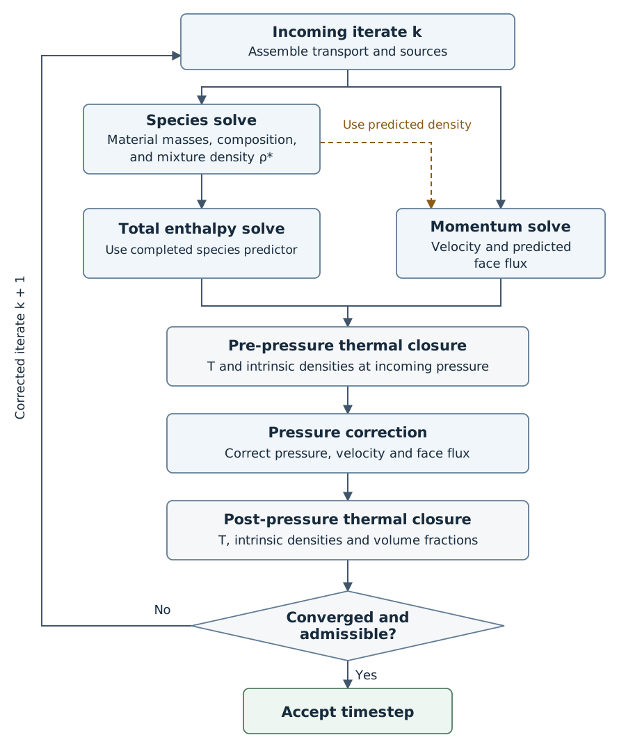
One nonlinear sweep. Species determines material masses, composition, and mixture density before the enthalpy solve. Momentum also uses that density when predictor gravity is enabled. Thermal closure precedes pressure correction and is repeated afterward. An unconverged state returns to the next sweep. — Fig. 16.11.1 Dependencies within one nonlinear sweep. The dashed arrow is the optional use of predicted mixture density in the paired momentum and face-flux gravity terms.#

16.11.1. Predictor updates#

Assemble species transport and its sources from the incoming iterate, using the linearization in Species Discretization. Each linear solve holds its coefficients and source fixed. The completed species predictor determines material masses, mixture density, and composition:

(16.11.1.1)#\[q_m^{*,k}=\sum_{s\in\mathcal K_m}z_{ms}^{*,k} \qquad \rho^{*,k}=\sum_m q_m^{*,k} \qquad \widetilde Y_s^{(m),*,k}=\frac{z_{ms}^{*,k}}{q_m^{*,k}} \quad(q_m^{*,k}>0)\]

Mixture density is therefore available before energy or pressure correction, without an EOS evaluation. Intrinsic material densities $\rho_m$ require the thermal closures below.

The energy solve accounts for the composition change at incoming pressure and temperature, together with an enthalpy-weighted species-residual correction. This couples the energy predictor to the new species state without changing the converged conservation equations. Its physical energy residual is retained for convergence checking. The correction uses incoming velocity; it does not depend on the momentum predictor. The derivation is in Material-to-energy predictor coupling.

The momentum predictor supplies velocity and the momentum-interpolated face volume flux. When gravity uses predicted density, both its cell force and paired face-flux contribution use $\rho^{*,k}$. This adds a species-to-momentum dependency. Other momentum density coefficients remain at the incoming iterate. Momentum and energy transport use the incoming mass flux in Eq. (16.8.1.1).

16.11.2. Pressure and thermal closure#

Before pressure correction, recover temperature from Eq. (16.3.1.6) using the predicted species, total enthalpy, and velocity at pressure $p^k$. Evaluate the intrinsic material densities $\rho_m^{\mathrm{pred},k}$, the material-volume error, and its fixed-enthalpy pressure response.

Solve the pressure-correction equation (16.7.3.2) using this volume error and the difference between the momentum and species predictor volume fluxes. Correct pressure, velocity, and face volume flux while holding $z_{ms}^{*,k}$ and $h_t^{*,k}$ fixed.

At the corrected pressure, recover temperature again with static enthalpy $h_t^{*,k}-\tfrac12\lVert\vec u^{\mathrm c,k}\rVert^2$. Reevaluate the intrinsic material densities and derive $\alpha_m^{k+1}=q_m^{*,k}/\rho_m^{k+1}$. Mixture density remains $\rho^{*,k}=\sum_m q_m^{*,k}$. The corrected face flux affects species transport on the next nonlinear sweep.

16.11.3. Convergence and acceptance#

Equation residuals, species and volume-fraction updates, material-volume closure, and corrected-flux continuity must satisfy their tolerances. The state must also satisfy the EOS, enthalpy closure, and volume-fraction bounds. The conservative species-update check is

(16.11.3.1)#\[\max_P \frac{\displaystyle\sum_m\sum_{s\in\mathcal K_m} \left|z_{ms,P}^{*,k}-z_{ms,P}^{k}\right|} {\max\!\left(\rho_P^{*,k},\rho_P^{k}\right)} \le\tau_z\]

Here $\tau_z$ is the species-update tolerance. Scaling by mixture density avoids division by a vanishing species or material mass. The continuity check uses the summed species flux at the corrected volume flow, with incoming donor and reconstruction coefficients held fixed:

(16.11.3.2)#\[\dot m_f^{\mathrm c,k} =\sum_m F_{q,m,f}^{*,k} +\left(\dot\Omega_f^{\mathrm c,k}-\dot\Omega_f^k\right) \sum_m\frac{\partial F_{q,m,f}}{\partial\dot\Omega_f}\]

A corrected flow that introduces an absent material also requires the appearance check in Eq. (16.15.3.4). If a check is unsatisfied, repeat with the corrected state as iterate $k+1$. Reaching an iteration limit does not establish convergence.

16.12. Advective Face Reconstruction#

These formulas supply the volume fraction, intrinsic density, and composition in Eq. (16.6.1.1). Volume fractions are reconstructed across materials. Density and composition are reconstructed within each present material. All inputs use the incoming nonlinear iterate; iteration superscripts are omitted in this section.

16.12.1. Volume fractions#

16.12.1.1. FOU and SOU volume-fraction candidates#

Use the stored face orientation from Loci Face Orientation and Cell Incidence. The donor $D$ is $\operatorname{cl}(f)$ for positive volume flow and $\operatorname{cr}(f)$ for negative flow; the other cell is the acceptor $A$. First-order upwinding (FOU) uses

(16.12.1.1)#\[\alpha_{m,f}^{FOU}=\alpha_{m,D}\]

Second-order upwinding (SOU) applies the scalar Barth limiter independently to each material volume fraction. With $\vec d_{Df}=\vec x_f-\vec x_D$, the tentative component slope is

(16.12.1.2)#\[r_{m,f} = \psi_{m,D}\nabla\alpha_{m,D}\mathbin{\cdot}\vec d_{Df}\]

The vector reconstruction applies its nonnegativity guards component by component:

(16.12.1.3)#\[\begin{split}s_{m,f}^{(1)} = \begin{cases} -\alpha_{m,D}, & \alpha_{m,D}+r_{m,f}<0,\\ r_{m,f}, & \text{otherwise} \end{cases} \qquad \bar s_{m,f} = \begin{cases} 0, & \alpha_{m,D}-\dfrac32s_{m,f}^{(1)}<0,\\ s_{m,f}^{(1)}, & \text{otherwise} \end{cases}\end{split}\]

The raw SOU candidate is

(16.12.1.4)#\[\alpha_{m,f}^{SOU,raw}=\alpha_{m,D}+\bar s_{m,f}\]

If $\alpha_{m,D}=0$, the guards set $\bar s_{m,f}=0$ for that component. Other components retain their own SOU candidates. The slope rescaling below then restores a zero sum of the complete slope vector.

16.12.1.2. MIG volume-fraction candidate#

MIG uses the normalized-variable-diagram (NVD) mapping of Thakur, Wright, and Neal [1]. During the coupled iteration, the EOS-derived fractions can sum to a value different from one. MIG first forms temporary fractions that partition each cell in the stencil:

(16.12.1.5)#\[\alpha_\Sigma=\sum_m\alpha_m \qquad \beta_m=\frac{\alpha_m}{\alpha_\Sigma}\]

Here $\alpha_\Sigma$ must be finite and positive. Boundary fractions are normalized in the same way. The usual discrete cell-gradient operator is then applied to these $\beta_m$ values to obtain $\nabla\beta_m$. Thus the values and gradients describe the same normalized field throughout the stencil. They satisfy $\sum_m\beta_m=1$ and, to roundoff, $\sum_m\nabla\beta_m=\vec0$, without changing the stored masses or EOS-derived cell fractions. Section Consistent material fractions for MIG reconstruction derives this construction and explains its effect on trace-material transport.

MIG then constructs a normalized-variable face value using a virtual upstream value bounded to the physical volume-fraction interval. This spatial NVD normalization is separate from the material normalization above. With $\vec r_{DA}=\vec x_A-\vec x_D$, define

(16.12.1.6)#\[\beta_{m,U}^{v} = \min\!\left(1,\max\!\left(0, \beta_{m,A} -2\nabla\beta_{m,D}\cdot\vec r_{DA} \right)\right) \qquad \widehat{\beta}_{m,D} = \frac{\beta_{m,D}-\beta_{m,U}^{v}} {\beta_{m,A}-\beta_{m,U}^{v}}\]

The bound and the normalization use the same upstream value. This prevents an out-of-range extrapolation from sustaining a finite outgoing fraction as the donor fraction vanishes. If the denominator is zero or the normalized donor falls outside $[0,1]$, use the donor value directly. Constant states also use that fallback.

The compressive IG branch is

(16.12.1.7)#\[\begin{split}\mathcal{I}(\xi) = \begin{cases} \xi, & \xi<0\ \text{or}\ \xi>1,\\ 3\xi-2\xi^2, & 0\le\xi<\tfrac12,\\ 1, & \tfrac12\le\xi\le1 \end{cases}\end{split}\]

Form the face gradient by opposite-volume weighting:

(16.12.1.8)#\[\nabla\beta_{m,f} = \frac{ \Omega_A\nabla\beta_{m,D}+\Omega_D\nabla\beta_{m,A} }{\Omega_D+\Omega_A} \qquad \gamma_f = \sqrt{ \left| \frac{\nabla\beta_{m,f}\cdot\vec r_{DA}} {\lVert\nabla\beta_{m,f}\rVert\lVert\vec r_{DA}\rVert} \right| } \qquad 0\le\gamma_f\le1\]

For a vanishing gradient or degenerate direction, set $\gamma_f=1$. MIG blends the compressive IG branch with the normalized identity mapping,

(16.12.1.9)#\[\mathcal{N}_{MIG}(\xi) = \gamma_f\mathcal{I}(\xi)+(1-\gamma_f)\xi \qquad \widehat\beta_{m,f}^{MIG} = \mathcal N_{MIG}(\widehat\beta_{m,D})\]

Alignment increases the contribution of the compressive IG branch; misalignment moves the candidate toward the donor value. Converting the normalized face value back to a volume fraction gives

(16.12.1.10)#\[\alpha_{m,f}^{MIG,raw} = \beta_{m,U}^{v} +\widehat{\beta}_{m,f}^{MIG} \left(\beta_{m,A}-\beta_{m,U}^{v}\right)\]

For an absent donor, $q_{m,D}=0$ and the raw candidate is $\alpha_{m,f}^{MIG,raw}=\beta_{m,D}=0$.

16.12.1.3. Preserving the volume-fraction sum#

Both SOU and MIG first produce componentwise candidates. Their slope balancing uses the donor value supplied to that reconstruction: the original fraction for SOU, and the temporary normalized fraction for MIG. Denote this base value by

(16.12.1.11)#\[a_{m,D}^{SOU}=\alpha_{m,D} \qquad a_{m,D}^{MIG}=\beta_{m,D}\]

For $X\in\{SOU,MIG\}$, define

(16.12.1.12)#\[\begin{split}\begin{aligned} s_{m,f}^{X} &= \alpha_{m,f}^{X,raw}-a_{m,D}^{X} \\ \Sigma_f^{X,-}&=\sum_m\min(0,s_{m,f}^{X}) \qquad \Sigma_f^{X,+}=\sum_m\max(0,s_{m,f}^{X}) \\ \Sigma_f^{X}&=\Sigma_f^{X,-}+\Sigma_f^{X,+} \end{aligned}\end{split}\]

The sign group responsible for a nonzero total slope is reduced:

(16.12.1.13)#\[\begin{split}\delta\alpha_{m,f}^{X} = \begin{cases} \displaystyle s_{m,f}^{X} \dfrac{\Sigma_f^{X,-}-\Sigma_f^{X}}{\Sigma_f^{X,-}} & \Sigma_f^{X}<0\ \text{and}\ s_{m,f}^{X}<0,\\[8pt] \displaystyle s_{m,f}^{X} \dfrac{\Sigma_f^{X,+}-\Sigma_f^{X}}{\Sigma_f^{X,+}} & \Sigma_f^{X}>0\ \text{and}\ s_{m,f}^{X}>0,\\[8pt] s_{m,f}^{X}, & \text{otherwise} \end{cases}\end{split}\]

Each active denominator is nonzero, and each applied factor lies in $[0,1]$. The final reconstructed volume fraction is

(16.12.1.14)#\[\alpha_{m,f}^{X}=a_{m,D}^{X}+\delta\alpha_{m,f}^{X} \qquad \sum_m\delta\alpha_{m,f}^{X}=0\]

The rescaling only moves a candidate slope toward zero. It therefore preserves each slope’s sign, any component bounds already satisfied by the base value and raw candidate, and the sum of the base values. An exact-zero candidate increment remains zero. Therefore,

(16.12.1.15)#\[\sum_m\alpha_{m,f}^{FOU} =\sum_m\alpha_{m,f}^{SOU} =\sum_m\alpha_{m,D} \qquad \sum_m\alpha_{m,f}^{MIG}=\sum_m\beta_{m,D}=1\]

If the base values and raw candidates lie in $[0,1]$ and the base values sum to one, the reconstructed fractions are nonnegative and sum to one. MIG meets this unit-sum condition through its temporary fractions; FOU and SOU retain any incoming donor sum error. Below, $\alpha_{m,f}$ denotes the selected FOU, SOU, or MIG result.

16.12.2. Density and composition within a material#

Material density, composition, and species enthalpies are defined only where the material is present. For a present donor, let $\mathcal S_m(D)=1$ when the material is also present throughout the donor’s one-ring gradient stencil. A conditional material scalar $\varphi_m$ then uses

(16.12.2.1)#\[\begin{split}\varphi_{m,f}^{SOU} = \begin{cases} \varphi_{m,D} +\psi_{\varphi_m,D}\nabla\varphi_{m,D}\mathbin{\cdot} (\vec x_f-\vec x_{D}), & \mathcal S_m(D)=1,\\[4pt] \varphi_{m,D}, & q_{m,D}>0\ \text{and}\ \mathcal S_m(D)=0 \end{cases}\end{split}\]

Composition uses the same support condition. Its SOU increments are rescaled to zero sum within each material, as defined in Eq. (16.12.2.6). When $q_{m,D}=0$, the reconstructed material mass is zero and no conditional material state is used.

16.12.2.1. Preserving the species sum#

For SOU, form the componentwise limited slope for every species in material $m$,

(16.12.2.2)#\[d_{ms,f} = \psi_{Y_{ms},D} \nabla\widetilde Y_{s,D}^{(m)}\mathbin{\cdot} (\vec x_f-\vec x_{D}) \qquad s\in\mathcal K_m\]

The vector-MUSCL positivity guards are applied component by component in two steps:

(16.12.2.3)#\[\begin{split}g_{ms,f}^{(1)} = \begin{cases} -\widetilde Y_{s,D}^{(m)}, & \widetilde Y_{s,D}^{(m)}+d_{ms,f}<0,\\[3pt] d_{ms,f}, & \text{otherwise} \end{cases} \qquad g_{ms,f} = \begin{cases} 0, & \widetilde Y_{s,D}^{(m)} -\dfrac{3}{2}g_{ms,f}^{(1)}<0,\\[5pt] g_{ms,f}^{(1)}, & \text{otherwise} \end{cases}\end{split}\]

The slope rescaling follows the volume-fraction construction above, now summing over the species of one material. Define

(16.12.2.4)#\[G_{m,f}=\sum_{s\in\mathcal K_m}g_{ms,f} \qquad G_{m,f}^{-}=\sum_{s\in\mathcal K_m}\min(0,g_{ms,f}) \qquad G_{m,f}^{+}=\sum_{s\in\mathcal K_m}\max(0,g_{ms,f})\]

Only the sign group responsible for a nonzero total slope is reduced:

(16.12.2.5)#\[\begin{split}\widehat g_{ms,f} = \begin{cases} \displaystyle g_{ms,f}\frac{G_{m,f}^{-}-G_{m,f}}{G_{m,f}^{-}}, &G_{m,f}<0\ \text{and}\ g_{ms,f}<0,\\[9pt] \displaystyle g_{ms,f}\frac{G_{m,f}^{+}-G_{m,f}}{G_{m,f}^{+}}, &G_{m,f}>0\ \text{and}\ g_{ms,f}>0,\\[9pt] g_{ms,f},&\text{otherwise} \end{cases}\end{split}\]

The active denominator in either rescaling branch is nonzero, and $\sum_{s\in\mathcal K_m}\widehat g_{ms,f}=0$. The face increment is therefore

(16.12.2.6)#\[\begin{split}\delta\widetilde Y_{ms,f} = \begin{cases} \widehat g_{ms,f}, & \text{SOU and } \mathcal S_m(D)=1,\\[4pt] 0, & \text{FOU or unsupported SOU stencil} \end{cases}\end{split}\]

The slope rescaling is applied independently to each material and preserves that material’s composition sum.

16.13. Diffusive Species Flux#

Species-dependent diffusivities can give a nonzero sum of Fick fluxes within a material. CMIM corrects this sum at each face so diffusion redistributes species without transporting material mass. The resulting flux is used in both the species and diffusive enthalpy equations.

For an internal face, let $L=\operatorname{cl}(f)$ and $R=\operatorname{cr}(f)$, with flux positive from $L$ to $R$. The material must be present in both cells. Its mixture-volume diffusion coefficient is $\Gamma_{ms}=q_mD^{\mathrm{eff}}_{ms}$. Using the center-to-face distance weight $\theta_f=d_{Lf}/(d_{Lf}+d_{Rf})$, take the harmonic face value

(16.13.1)#\[\begin{split}\Gamma_{ms,f}^{H} =\begin{cases} \displaystyle \left[\frac{\theta_f}{\Gamma_{ms,L}} +\frac{1-\theta_f}{\Gamma_{ms,R}}\right]^{-1}, & q_{m,L},q_{m,R},\Gamma_{ms,L},\Gamma_{ms,R}>0\\[6pt] 0, & \text{otherwise} \end{cases}\end{split}\]

Use the face-area decomposition $\vec S_f=\mathcal G_f(\vec x_R-\vec x_L)+\vec T_f$ from Eq. (4.2.1.16). The raw two-point conductance is $\widehat G_{ms,f}=\mathcal G_f\Gamma_{ms,f}^{H}$, in $\mathrm{kg/s}$. For a one-species material the composition is identically one; set its conductance and diffusion flux to zero.

When the material is present throughout both cells’ gradient stencils, interpolate its composition gradient using opposite-cell-volume weights:

(16.13.2)#\[\overline{\nabla\widetilde Y}^{(m)}_{s,f} =\frac{\Omega_R\nabla\widetilde Y^{(m)}_{s,L} +\Omega_L\nabla\widetilde Y^{(m)}_{s,R}}{\Omega_L+\Omega_R}\]

The same stencil and weights apply to every species of the material. The raw diffusive mass flow is

(16.13.3)#\[\widehat F_{ms,f} =\widehat G_{ms,f}\left(\widetilde Y^{(m)}_{s,L}-\widetilde Y^{(m)}_{s,R}\right) -\Gamma_{ms,f}^{H}\overline{\nabla\widetilde Y}^{(m)}_{s,f}\cdot\vec T_f\]

If either gradient stencil lacks material support, omit the nonorthogonal term. If the material is absent in either adjacent cell, the entire flux is zero without evaluating a conditional composition or gradient.

To correct the species sum, collect the positive and negative raw flux magnitudes within each material:

(16.13.4)#\[P_{m,f}=\sum_{s\in\mathcal K_m}[\widehat F_{ms,f}]^+ \qquad N_{m,f}=\sum_{s\in\mathcal K_m}[-\widehat F_{ms,f}]^+\]

Here $[a]^+=\max(a,0)$. Reduce the group with the larger magnitude:

(16.13.5)#\[\begin{split}F_{ms,f} =\begin{cases} \displaystyle\frac{N_{m,f}}{P_{m,f}}\widehat F_{ms,f}, & \widehat F_{ms,f}>0\ \text{and}\ P_{m,f}>N_{m,f}\\[6pt] \displaystyle\frac{P_{m,f}}{N_{m,f}}\widehat F_{ms,f}, & \widehat F_{ms,f}<0\ \text{and}\ N_{m,f}>P_{m,f}\\[6pt] \widehat F_{ms,f}, & \text{otherwise} \end{cases}\end{split}\]

Each active denominator is positive. The correction acts on the complete raw flux, including its nonorthogonal part. It reduces magnitudes without reversing signs and enforces the zero-sum condition in Eq. (16.6.1.3), to roundoff.

Apply the same factor to $\widehat G_{ms,f}$ to obtain the conductance $G_{ms,f}$ used in the implicit species update. If the raw flux is zero, leave its conductance unchanged. Both the factor and the corrected conductance remain fixed during the linear solve.

Material presence in adjacent cells does not establish connectivity of the material portions inside them. Overlapping volume-fraction tails can therefore activate diffusion links; this approximation depends on the resolved interface thickness. At an impermeable wall the normal species flux is zero. Prescribed inflow composition sets advection; a nonzero boundary diffusion flux requires a separate closure.

16.14. Chemistry Integration#

For unsplit chemistry, the source in the species predictor is $\alpha_m\dot\omega_s^{(m)}=(q_m/\rho_m)\dot\omega_s^{(m)}$. Since $\widetilde Y_s^{(m)}=z_{ms}/q_m$, its destruction coefficient in Eq. (16.6.2.3) is

(16.14.1)#\[\ell_{ms}^k =\max\!\left(0,-\frac{1}{\rho_m^k} \frac{\partial\dot\omega_s^{(m)}}{\partial\widetilde Y_s^{(m)}}\bigg|_k\right)\]

The derivative holds $q_m$, $\rho_m$, pressure, temperature, and the other species fractions fixed. The coefficient has units of $\mathrm{s^{-1}}$; it is zero for absent materials and wholly explicit sources.

Split chemistry instead integrates the cell reactions over $\Delta t$ from the accepted state, at fixed volume and internal energy. The transport step uses the reaction endpoint $z_{ms}^{\mathrm{chem}}$ as its BDF1 history:

(16.14.2)#\[\frac{\Omega_P}{\Delta t} \left(z_{ms,P}^{*,k}-z_{ms,P}^{\mathrm{chem}}\right) +\sum_{f\in\mathcal F_P}\sigma_{Pf} \left(F_{z,ms,f}^{*,k}+F_{ms,f}^{\mathrm{lin},*,k}\right) =\Omega_P S_{ms,P}^{\mathrm{tr,rem},k}\]

Here $S_{ms}^{\mathrm{tr,rem}}$ contains only transfer sources not included in the reaction integration. Chemistry is not added again as a source. Reactions within a material conserve its mass; reactions between materials may change their individual masses while preserving the total. The species reference energies contain reaction heat, so the total-energy history stays unchanged. This is first-order source splitting.

16.15. Material-Appearance Face Reference#

This section applies Material appearance to one material $m$ at an internal face. An empty cell means empty of material $m$; other materials still occupy the cell. Local material presence does not by itself establish that a wider reconstruction stencil supports that material.

16.15.1. One oriented internal face#

Let $P=L_f$ and $N_f=R_f$, with $\mathbf S_f$ pointing from $P$ to $N_f$. For all four sketches, take $\dot{\Omega}_f^k<0$. The donor is then $D_f^k=N_f$, and a negative material mass flux is inflow to $P$:

(16.15.1.1)#\[\dot{\Omega}_f^k=\mathbf u_f^k\mathbin{\cdot}\mathbf S_f, \qquad \dot m_{m,f}^k=\widehat q_{m,f}^k\dot{\Omega}_f^k.\]

Here $\widehat q_{m,f}^k$ is the selected material face density. In standard mode it equals the reconstructed $\alpha_{m,f}^k\rho_{m,f}^k$ for a present donor and is zero for an absent donor.

16.15.1.1. Material absent from both cells#

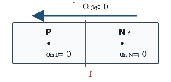
$Adjacent cells P and N f share face f. Cell-center dots mark P and N f, and material m has zero volume fraction in both cells.$

Fig. 16.15.1.1 Material $m$ is absent at both cell centers.#

The donor is empty, so $\alpha_{m,f}^k=\widehat q_{m,f}^k=0$. The incoming state gives no advective material, species, or enthalpy flux for $m$ at this face. History, sources, or another face may still supply species during the implicit solve.

16.15.1.2. Material present only in the receiver#

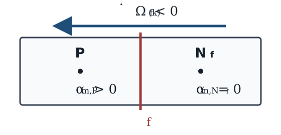
$Adjacent cells P and N f share face f. Cell-center dots mark P and N f. Material m has positive volume fraction in P and zero volume fraction in N f.$

Fig. 16.15.1.2 Material $m$ is present in receiver $P$ and absent from donor $N_f$.#

The empty donor again gives $\alpha_{m,f}^k=\widehat q_{m,f}^k=0$. This face supplies no incoming-state inflow of $m$. Material already in $P$, its accepted history, and its local sources remain in the cell balance. Reversing the volume flux would make $P$ the donor.

16.15.1.3. Material present in both cells#

$Adjacent cells P and N f share face f. Cell-center dots mark P and N f, and material m has positive volume fraction in both cells.$

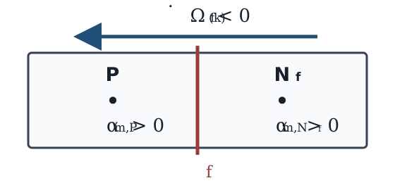
Fig. 16.15.1.3 Material $m$ is present at both cell centers.#

With FOU reconstruction, $\widehat q_{m,f}^k=q_{m,N_f}^k$. A higher-order VOF scheme may give a different material face density. SOU density, composition, and species enthalpy require material support throughout the donor’s gradient stencil, not just in these two cells. For $\widehat q_{m,f}^k>0$, the negative volume flux carries material into $P$.

16.15.1.4. Material present only in the donor#

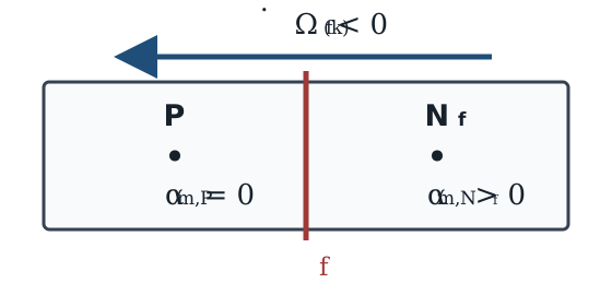
$Adjacent cells P and N f share face f. Cell-center dots mark P and N f. Material m has zero volume fraction in P and positive volume fraction in N f.$

Fig. 16.15.1.4 Material $m$ is absent from receiver $P$ and present in donor $N_f$.#

This is the appearance case. The VOF scheme supplies the material face fraction. Density, composition, and species enthalpies use donor values because the conditional-state stencil crosses into a cell where material $m$ is absent. The species equations carry these donor species into $P$ through their common material coefficient.

No receiver composition or intrinsic density is needed by this advective flux. Once the species predictor has a positive material sum, its composition and the common pressure and temperature define the new receiver EOS state.

Reversing $\dot{\Omega}_f^k$ interchanges donor and receiver. At zero volume flux, the incoming-state advective flux is zero.

16.15.2. Lagged face states and the implicit species solve#

An absent lagged donor does not force the implicit predictor flux to remain zero throughout the global solve. For $q_{m,D_f^k}^k=0$, Eq. (16.16.1.9) gives

(16.15.2.1)#\[F_{z,ms,f}^{*,k}=\dot{\Omega}_f^kz_{ms,D_f^k}^{*,k}, \qquad F_{q,m,f}^{*,k} =\sum_{s\in\mathcal K_m}F_{z,ms,f}^{*,k} =\dot{\Omega}_f^kq_{m,D_f^k}^{*,k}.\]

Another incoming face can make the donor species predictor positive. The same implicit coupling can then transport species through this face and through several cells that were empty in the incoming iterate. Material mass follows from the species sum at every stage.

The reconstructed coefficients and enthalpy fluxes remain lagged during the predictor solves and are rebuilt at the next outer iteration. At convergence, incoming and predicted states agree. A donor that remains exactly empty then has zero material, species, and enthalpy flux.

16.15.3. The appearing material in the pressure row#

After the species solve, derive $q_{m,P}^{*,k}=\sum_s z_{ms,P}^{*,k}$. If this sum is zero, the material does not contribute to the cell’s predicted volume or pressure response. If it is positive, its composition is $z_{ms,P}^{*,k}/q_{m,P}^{*,k}$, and the pre-pressure closure supplies $\rho_{m,P}^{\mathrm{pred},k}$.

The pressure response follows the selected species linearization. With implicit material advection and a present lagged donor,

(16.15.3.1)#\[\frac{\partial F_{q,m,f}}{\partial\dot{\Omega}_f} = \frac{\widehat q_{m,f}^k}{q_{m,N_f}^k}q_{m,N_f}^{*,k}.\]

For an absent lagged donor it is $q_{m,N_f}^{*,k}$. Standard deferred material advection uses $q_{m,N_f}^{*,k}$ for either donor state, as in Eq. (16.16.1.11). The row’s volume-flux weight is therefore

(16.15.3.2)#\[\begin{split}W_{P,f}^k = \sum_{\substack{m\\q_{m,P}^{*,k}>0}} \frac{1}{\rho_{m,P}^{\mathrm{pred},k}} \frac{\partial F_{q,m,f}}{\partial\dot{\Omega}_f}.\end{split}\]

The receiver density converts the material mass-flux response to a volume-flux response. The cell source is the predicted volume error

(16.15.3.3)#\[\begin{split}E_{V,P}^{\mathrm{pred},k} = \sum_{\substack{m\\q_{m,P}^{*,k}>0}} \frac{q_{m,P}^{*,k}}{\rho_{m,P}^{\mathrm{pred},k}}-1.\end{split}\]

Both use the species-derived material masses and their predicted EOS states. The species densities, material reconstruction coefficient, and explicit composition correction stay fixed during pressure correction. The cell thermodynamic response is the fixed-enthalpy derivative in Eq. (16.7.1.3).

Pressure correction can activate a zero-flow face or reverse its donor. If the new inflow carries a material absent from the predicted receiving cell, another species update is needed. Let $\mathcal F_{P,m}^{\mathrm{app}}$ contain those incoming internal faces for material $m$ in cell $P$. Estimate their volume-fraction change from the corrected donors:

(16.15.3.4)#\[\Delta\alpha_{\mathrm{app},P,m}^k =\frac{\Delta t}{\Omega_P} \sum_{f\in\mathcal F_{P,m}^{\mathrm{app}}} |\dot\Omega_f^{\mathrm c,k}| \frac{q_{m,D_f}^{*,k}}{\rho_{m,D_f}^{\mathrm{pred},k}}\]

Here $D_f$ is selected by the corrected flux, and only present donor states are evaluated. At a newly incoming boundary, use the prescribed material volume fraction instead of the donor ratio. The maximum over cells and materials must satisfy the material-update tolerance before accepting the time step. Otherwise another species update and thermal closure are needed.

16.15.4. Composition supplied by inflow#

Consider a converged, source-free, diffusion-free FOU state with no accepted history of material $m$ in cell $P$. Its incoming species fluxes give

(16.15.4.1)#\[\widetilde{\mathbf Y}_{P}^{(m)} = \frac{ \sum_f F_{q,m,Pf}^{\mathrm{in}}\widetilde{\mathbf Y}_{D_f}^{(m)} }{ \sum_f F_{q,m,Pf}^{\mathrm{in}} }, \qquad F_{q,m,Pf}^{\mathrm{in}} =\max\!\left(-\sigma_{Pf}F_{q,m,f},0\right),\]

provided the denominator is positive. One inflow supplies its donor composition; several inflows supply their material-mass-flux-weighted composition. This follows by summing the species rows and dividing each species balance by their material sum. Accepted history adds its own mass weight. A source that creates material supplies the species and energy contributions specified by its physical model.

During the iteration, the composition is always derived from the local species predictor and its sum. It is not assigned from a selected neighbor.

16.15.5. Operator behavior near material absence#

Operation	Treatment
Species advection	Use the common material coefficient in every owned species row. Retain implicit FOU coupling for an absent lagged donor.
Material face reconstruction	Reconstruct the derived volume fractions. FOU, guarded SOU, and MIG leave an exactly absent donor component at zero.
Density and species-enthalpy SOU	Extrapolate only with material present throughout the donor’s gradient stencil; otherwise use the donor value.
Composition SOU	Apply the same support condition and preserve zero-sum increments separately within each material.
Species diffusion	Require material in both adjacent cells. Retain the compact term but omit the nonorthogonal correction if the wider gradient stencil is unsupported.
Pressure-volume closure	Use positive species sums and their predicted EOS states. An absent material contributes zero volume.
Pressure face response	Convert the summed species mass-flux response to cell volume using the active predicted cell density.

In an admissible state, exact absence means that every species density of the material is zero. A positive material sum instead defines a composition and requires an EOS state, however small that sum is.

16.15.6. Material cutoff#

Setting a material’s negligible positive density to zero also sets all its species densities to zero. Individual trace species within a retained material are preserved. For an effective density cutoff $q_c$, the removed mass is less than $q_c\Omega_P$ per material, cell, and removal operation. This is a nonconservative approximation: retaining velocity and specific total enthalpy while reducing mass also changes momentum and total energy. The cutoff must be small relative to the physical material densities, and the accumulated removal must be included when assessing conservation.

16.16. Transport Formulations and Experimental Extensions#

The species equations advance $z_{ms}$, their sums give $q_m$, and the energy equation advances mixture total enthalpy $h_t$. In the segregated iteration of Segregated Nonlinear Algorithm, each predictor uses coefficients and face reconstructions from the same incoming state. The predictors become mutually consistent as the outer iterations converge.

Four changes to this process are considered here. They address different questions:

Approach	Question addressed	What changes
Implicit material advection	How should a reconstructed material flux enter the species equation?	Part of the explicit correction becomes a coefficient of the unknown species density
Conservative flux rescaling	How much of a face correction can be applied without exhausting a cell’s available mass?	Material and composition corrections are reduced by shared face factors
Material-to-energy coupling	How should the energy predictor account for a change in composition?	The completed species predictor supplies a correction to the energy update
Consistent MIG reconstruction	How should an incompletely converged material-volume sum affect the reconstructed interface?	Temporary fractions and gradients satisfy the material-volume identities before reconstruction

The first two are available transport formulations. Consistent reconstruction is part of the current MIG scheme. Material-to-energy coupling makes the energy predictor depend on the completed species predictor; MIG reconstruction retains the incoming Picard state. The notation retains superscript $n$ for the accepted time level, $k$ for the incoming outer iterate, and $*,k$ for the predictor result. The species index is $s\in\mathcal K_m$.

16.16.1. Implicit material advection#

Consider the convective flux of one species of one material through an internal face. Write $F_f$ for its mass flow rate and $z$ for its mass per mixture volume, suppressing the material and species indices in this derivation. The donor $D=D_f^k$ is selected by the incoming volume flow $\dot{\Omega}_f^k$. Superscript $k$ marks known values from the incoming iteration; $*,k$ marks the unknown predictor. The standard deferred flux from Eq. (16.6.2.1) is

(16.16.1.1)#\[F_f^{\mathrm{std},*,k} =\dot{\Omega}_f^k \left[z_D^{*,k}+\left(z_f^k-z_D^k\right)\right]\]

Here $z_f^k$ is the reconstructed face value. The donor term is implicit, while the correction $z_f^k-z_D^k$ stays fixed during the linear solve. If that correction removes more species than a cell’s history and inflow can supply, the solved cell value can become negative. Implicit material advection changes the treatment of the material part of this correction.

16.16.1.1. Separate material transport from composition transport#

For a material present in the donor, the species density is $z=qY$. Here $q=\alpha\rho$ is material mass per mixture volume, with $\rho$ the intrinsic material density. The species mass fraction within that material is $Y$, abbreviating $\widetilde Y_s^{(m)}$. At the face, $q_f^k$ denotes the reconstructed material density, and $Y_f^k$ denotes the reconstructed composition. When distinguishing these from rescaled values below, write $q_{m,f}^{\mathrm{rec},k}$ and $\widehat Y_{ms,f}^k$, respectively. Thus $z_f^k=q_f^kY_f^k$ and $z_D^k=q_D^kY_D^k$. Adding and subtracting $q_f^kY_D^k$ splits the face correction into two parts:

(16.16.1.2)#\[\begin{split}\begin{aligned} z_f^k-z_D^k &=q_f^kY_f^k-q_D^kY_D^k\\ &=\left(q_f^k-q_D^k\right)Y_D^k +q_f^k\left(Y_f^k-Y_D^k\right) \end{aligned}\end{split}\]

The first part changes how much material crosses the face at the donor composition. The second changes the species proportions of that material flow. Substituting both parts back into the full flux gives

(16.16.1.3)#\[F_f^{\mathrm{std},*,k} =\dot{\Omega}_f^k \left[ z_D^{*,k} +\underbrace{\left(q_f^k-q_D^k\right)Y_D^k}_{\text{material correction}} +\underbrace{q_f^k\left(Y_f^k-Y_D^k\right)}_{\text{composition correction}} \right]\]

This is still the standard deferred flux. Both corrections are known during the solve.

16.16.1.2. Make the material correction implicit#

Assume the donor contains the material, so $q_D^k>0$. In the material correction, use $Y_D^k=z_D^k/q_D^k$:

(16.16.1.4)#\[\left(q_f^k-q_D^k\right)Y_D^k =\frac{q_f^k-q_D^k}{q_D^k}z_D^k\]

This equality only rewrites the known material correction. The alternative linearization now replaces its final $z_D^k$ by the unknown $z_D^{*,k}$. The ratio stays fixed, and the composition correction is unchanged. This replacement is a numerical choice, not an algebraic identity. The full modified flux is

(16.16.1.5)#\[F_f^{\mathrm{imp},*,k} =\dot{\Omega}_f^k \left[ z_D^{*,k} +\frac{q_f^k-q_D^k}{q_D^k}z_D^{*,k} +q_f^k\left(Y_f^k-Y_D^k\right) \right]\]

The first two terms now contain the same unknown. Their coefficients combine as

(16.16.1.6)#\[1+\frac{q_f^k-q_D^k}{q_D^k} =\frac{q_f^k}{q_D^k}\]

The resulting implicit material-advection flux is therefore

(16.16.1.7)#\[F_f^{\mathrm{imp},*,k} =\dot{\Omega}_f^k\frac{q_f^k}{q_D^k}z_D^{*,k} +\dot{\Omega}_f^k q_f^k\left(Y_f^k-Y_D^k\right)\]

The material contribution now responds to the unknown species density during the solve. The composition correction remains explicit. The ratio $q_f^k/q_D^k$ uses incoming values and is held fixed, as are the other Picard coefficients. It is common to all species of the material.

16.16.1.3. Checks on the resulting flux#

With FOU material reconstruction, $q_f^k=q_D^k$. The coefficient ratio is one, the material correction is zero, and the standard and implicit formulations coincide at every iteration.

At nonlinear convergence, $z_D^{*,k}=z_D^k=q_D^kY_D^k$. Substituting into the final flux gives

(16.16.1.8)#\[F_f^{\mathrm{imp}} =\dot{\Omega}_f q_fY_D +\dot{\Omega}_f q_f\left(Y_f-Y_D\right) =\dot{\Omega}_f q_fY_f =F_f^{\mathrm{std}}\]

The iteration superscripts have been dropped in this converged expression. Both formulations recover the same reconstructed species flux; they differ in how the linear solves approach it.

For nonnegative $q_f^k$, the modified coefficient retains the upwind sign. With FOU composition, $Y_f^k=Y_D^k$, so the remaining explicit correction also vanishes. SOU composition can still supply a correction, and diffusion and sources retain their own admissibility requirements. The change removes the deferred material contribution as a source of negative predictors, but is not a general positivity guarantee for the species equation.

16.16.1.4. Selected face density and absent donors#

Restore the material and species indices for the following relations. The explicit composition term is $\delta F_{z,ms,f}^k=\dot{\Omega}_f^k q_{m,f}^{\mathrm{rec},k} \delta\widetilde Y_{ms,f}^k$, where $\delta\widetilde Y_{ms,f}^k=\widehat Y_{ms,f}^k-\widetilde Y_{s,D}^{(m),k}$. This increment sums to zero within each material. At an absent donor the correction is zero without evaluating a composition.

Conservative rescaling replaces $q_{m,f}^{\mathrm{rec},k}$ by $\widehat q_{m,f}^k$ in the material correction or its implicit coefficient. It also bounds $\delta F_{z,ms,f}^k$, as derived in Conservative flux rescaling. Without rescaling, $\widehat q_{m,f}^k=q_{m,f}^{\mathrm{rec},k}$ and the formulas above apply directly. With rescaling, their equivalence at convergence holds for the same selected face density and composition correction.

At an absent donor, $q_{m,D}^k=\widehat q_{m,f}^k=0$. Both formulations retain $\dot{\Omega}_f^k z_{ms,D}^{*,k}$ without evaluating a composition or dividing by zero. Material supplied through another face can still pass through the implicit stencil. Including this branch, the implicit material flux used in the species row is

(16.16.1.9)#\[\begin{split}F_{z,ms,f}^{\mathrm{imp},*,k} =\begin{cases} \displaystyle \dot{\Omega}_f^k\frac{\widehat q_{m,f}^k}{q_{m,D}^k} z_{ms,D}^{*,k}+\delta F_{z,ms,f}^k, & q_{m,D}^k>0\\[6pt] \dot{\Omega}_f^k z_{ms,D}^{*,k}, & q_{m,D}^k=0 \end{cases}\end{split}\]

Summing over species cancels the composition correction and gives the material predictor flux:

(16.16.1.10)#\[\begin{split}F_{q,m,f}^{\mathrm{imp},*,k} \equiv\sum_{s\in\mathcal K_m}F_{z,ms,f}^{\mathrm{imp},*,k} =\begin{cases} \displaystyle \dot{\Omega}_f^k\frac{\widehat q_{m,f}^k}{q_{m,D}^k} q_{m,D}^{*,k}, & q_{m,D}^k>0\\[6pt] \dot{\Omega}_f^k q_{m,D}^{*,k}, & q_{m,D}^k=0 \end{cases}\end{split}\]

Here $q_{m,D}^{*,k}=\sum_s z_{ms,D}^{*,k}$. At convergence this becomes $F_{q,m,f}=\dot{\Omega}_f\widehat q_{m,f}$, as does the standard material flux with the same rescaling.

16.16.1.5. Consistent pressure response#

Pressure correction changes the face volume flow. Its material response must follow the chosen species linearization. Hold the predicted densities, the deferred corrections, and the reconstructed ratio fixed while changing $\dot{\Omega}_f$. For a present donor, the responses of the summed species rows are

(16.16.1.11)#\[\left.\frac{\partial F_{q,m,f}}{\partial\dot{\Omega}_f}\right|_{\mathrm{std}} =q_{m,D}^{*,k}, \qquad \left.\frac{\partial F_{q,m,f}}{\partial\dot{\Omega}_f}\right|_{\mathrm{imp}} =\frac{\widehat q_{m,f}^k}{q_{m,D}^k}q_{m,D}^{*,k}\]

The absent-donor response is $q_{m,D}^{*,k}$ for either formulation. These are responses of the frozen predictor rows, not full derivatives of the converged reconstructed flux. The standard branch in Eq. (16.7.2.1) holds its entire deferred material mass-flow correction fixed along with its composition correction.

16.16.2. Conservative flux rescaling#

Conservative rescaling reduces face corrections before they enter the cell balances. One shared factor is used on both sides of an internal or periodic face, so the flux remains equal and opposite in the neighboring cells. No species inventory is changed independently after the solve.

The basic bound compares a proposed loss with the mass available to support it. For example, if a cell contains $2\ \mathrm{mg}$ of a species at the accepted time level and its outgoing correction would remove $3\ \mathrm{mg}$ during the next step, an inventory-only bound permits at most two-thirds of that correction. Other faces and the implicit solve may supply mass, but this initial bound does not rely on that replenishment.

The construction applies this idea in two stages. First limit the material correction distributed at donor composition. Then limit the composition correction using what remains on the species right-hand side. A bound on their initial sum is insufficient: an outward material correction and an inward composition correction may cancel. Reducing only the latter would increase the net outgoing loss.

16.16.2.1. Common material reconstruction factor#

The material part of Eq. (16.16.1.2) gives the unlimited material correction and its species shares at iterate $k$:

(16.16.2.1)#\[\Delta F_{q,m,f}^k =\dot{\Omega}_f^k\left(q_{m,f}^{\mathrm{rec},k}-q_{m,D_f^k}^k\right), \qquad \Delta F_{z,ms,f}^{q,k} =\Delta F_{q,m,f}^k\widetilde Y_{ms,D_f^k}^{(m),k}\]

Both corrections are zero at an absent donor without evaluating its composition. Their species sum is the material correction. The same inventory calculation is applied to every $q_m$ and every $z_{ms}$. For that calculation, use $c$ to label any one of these components and $Q_{P,c}^n$ for its nonnegative accepted density. Its correction is $\Delta F_q$ for a material or $\Delta F_z^q$ for a species.

For fixed volumes and BDF1, define the total outgoing correction rate $L_{P,c}^k$ and available inventory rate $A_{P,c}^n$:

(16.16.2.2)#\[L_{P,c}^k =\sum_{f\in\mathcal F_P^{\mathrm{int}}} \max\!\left(\sigma_{Pf}\Delta F_{c,f}^k,0\right), \qquad A_{P,c}^n=\frac{\Omega_P}{\Delta t}Q_{P,c}^n\]

The factor $\sigma_{Pf}$ converts the stored face orientation to outward from cell $P$, as in Loci Face Orientation and Cell Incidence. Taking the positive part counts only correction fluxes that remove mass from $P$. The set $\mathcal F_P^{\mathrm{int}}$ includes internal and periodic faces. A correction can oppose the carrier volume flux, so its own sign determines which cell loses mass.

Both $L$ and $A$ have units of mass per time. In particular, $A$ is the accepted-history contribution from the BDF1 row, rather than the mass itself. The ratio $A/L$ gives the permitted fraction of the outgoing correction:

(16.16.2.3)#\[\begin{split}\eta_{P,c}^k =\begin{cases} 1, & L_{P,c}^k=0\\ \displaystyle\min\!\left(1,\frac{A_{P,c}^n}{L_{P,c}^k}\right), & L_{P,c}^k>0 \end{cases}\end{split}\]

Choose one cell factor that satisfies every component’s bound. Then use the smaller factor from the two cells sharing the face:

(16.16.2.4)#\[\eta_P^k=\min_c\eta_{P,c}^k, \qquad \eta_f^k=\min\!\left(\eta_{\operatorname{cl}(f)}^k, \eta_{\operatorname{cr}(f)}^k\right)\]

Here $0\le\eta_f^k\le1$. A value of one retains the full material correction, and zero removes it. The limited outgoing loss of every component is at most its accepted inventory rate. The same factor applies to every material and species at that face. In floating-point arithmetic, a small relative roundoff margin is reserved in the allowance and active ratios are rounded toward zero. This protects the bound when separate face products are summed; it is not a floor on the transported density.

The resulting material face density is

(16.16.2.5)#\[\widehat q_{m,f}^k =(1-\eta_f^k)q_{m,D_f^k}^k+\eta_f^k q_{m,f}^{\mathrm{rec},k}\]

Thus $\eta_f^k=0$ gives the donor value, while $\eta_f^k=1$ gives the reconstructed value. This nonnegative blend replaces $q^{\mathrm{rec}}$ in the material correction of Eq. (16.16.1.3), or in the coefficient of Eq. (16.16.1.7) (where the reconstructed density is abbreviated as $q_f^k$). Because the factor is the minimum over all components, a species present in only a small amount can restrict the material correction for the entire face.

16.16.2.2. Material-local composition factor#

After fixing the material factor, the proposed composition correction is

(16.16.2.6)#\[\Delta F_{z,ms,f}^{Y,k} =\eta_f^k\dot{\Omega}_f^k q_{m,f}^{\mathrm{rec},k} \delta\widetilde Y_{ms,f}^k\]

Its species sum within each material is zero. The factor $\eta_f^k$ already reduces this correction along with the material reconstruction. The second stage can reduce it further to protect each species.

Recall the species row in Eq. (16.6.2.5), with under-relaxation included. Define ${}^{(z)}\!b_{ms,P,0}^k$ as its assembled right-hand side before adding the composition correction; the subscript $0$ identifies this stage, not a time level. Adding the correction produces

(16.16.2.7)#\[{}^{(z)}\!b_{ms,P}^k ={}^{(z)}\!b_{ms,P,0}^k -\sum_{f\in\mathcal F_P^{\mathrm{int}}} \sigma_{Pf}\delta F_{z,ms,f}^k\]

An outgoing correction is subtracted from the right-hand side; an incoming one adds to it. The remaining allowance is the nonnegative part of ${}^{(z)}\!b_{ms,P,0}^k$ available for outgoing composition correction. It is a mass rate, like the other terms in the species row, and it is not the completed species solution.

This allowance depends on which material linearization was assembled. Let $B_{ms,P}^k$ collect the accepted temporal history, physical sources, boundary inflow, and deferred diffusion terms. Let ${}^{(z)}\!a_{ms,P}^{\mathrm{std},k}$ and ${}^{(z)}\!a_{ms,P}^{\mathrm{imp},k}$ denote the respective unrelaxed diagonals. Using the under-relaxation contribution from Segregated Nonlinear Algorithm, with $0<\alpha_z\le1$, gives

(16.16.2.8)#\[\begin{split}\begin{aligned} {}^{(z)}\!b_{ms,P,0}^{\mathrm{std},k} &=B_{ms,P}^k +\frac{1-\alpha_z}{\alpha_z} {}^{(z)}\!a_{ms,P}^{\mathrm{std},k}z_{ms,P}^k -\sum_{f\in\mathcal F_P^{\mathrm{int}}} \sigma_{Pf}\eta_f^k\Delta F_{z,ms,f}^{q,k}\\ {}^{(z)}\!b_{ms,P,0}^{\mathrm{imp},k} &=B_{ms,P}^k +\frac{1-\alpha_z}{\alpha_z} {}^{(z)}\!a_{ms,P}^{\mathrm{imp},k}z_{ms,P}^k \end{aligned}\end{split}\]

The standard row includes the signed material correction. The implicit row already contains it in its matrix. Relaxation must use that same matrix’s diagonal. The allowance therefore accounts for the material, diffusion, and source terms already assembled; the composition correction cannot be assigned the full temporal inventory again. Different linearizations can give different allowances and limiter factors, even though their fluxes agree at convergence when the factors are the same.

Count the proposed outgoing composition corrections in the same way as the material corrections:

(16.16.2.9)#\[L_{P,ms}^{Y,k} =\sum_{f\in\mathcal F_P^{\mathrm{int}}} \max\!\left(\sigma_{Pf}\Delta F_{z,ms,f}^{Y,k},0\right)\]

Within each material, the most restrictive species determines a common composition factor:

(16.16.2.10)#\[\begin{split}\eta_{Y,m,P}^k =\min\!\left( 1,\min_{\substack{s\in\mathcal K_m\\L_{P,ms}^{Y,k}>0}} \frac{\max\!\left({}^{(z)}\!b_{ms,P,0}^k,0\right)}{L_{P,ms}^{Y,k}} \right)\end{split}\]

If there is no positive outgoing composition rate, the factor is one. The face factor and the final composition correction are

(16.16.2.11)#\[\eta_{Y,m,f}^k =\min\!\left(\eta_{Y,m,\operatorname{cl}(f)}^k, \eta_{Y,m,\operatorname{cr}(f)}^k\right)\]

(16.16.2.12)#\[\delta F_{z,ms,f}^k =\eta_{Y,m,f}^k\Delta F_{z,ms,f}^{Y,k}\]

Every species in material $m$ uses the same face factor, preserving the zero sum. Different materials may use different composition factors. The outgoing correction obeys

(16.16.2.13)#\[\sum_{f\in\mathcal F_P^{\mathrm{int}}} \max\!\left(\sigma_{Pf}\delta F_{z,ms,f}^k,0\right) \le\eta_{Y,m,P}^k L_{P,ms}^{Y,k} \le\max\!\left({}^{(z)}\!b_{ms,P,0}^k,0\right)\]

If the pre-correction allowance is nonnegative, the final right-hand side remains nonnegative: the outgoing loss is bounded, and incoming corrections only add to it. The species row explains why this helps. With a positive diagonal, nonnegative neighbor coefficients, and a nonnegative right-hand side, updating a cell from nonnegative neighbor values gives a nonnegative species density. Gauss–Seidel sweeps starting from nonnegative values preserve this property. If those sweeps converge, the linear solution is also nonnegative; the limiter alone does not establish their convergence.

A sufficient bound, not a universal positivity guarantee

A finite negative allowance is not itself a negative species solution. Implicit neighbor inflow can compensate for a negative local right-hand side. The limiter suppresses outgoing composition corrections when that species has no positive allowance, but it cannot guarantee positivity of the whole row in this situation. The completed species predictor still needs an admissibility check. Nonfinite allowances are invalid.

This BDF1 inventory argument does not establish bounds for higher-order time integration, arbitrary sources, or deferred diffusion. It also does not establish nonlinear convergence or the EOS-derived volume-fraction bounds. The face budget above covers internal and periodic corrections. An open boundary with a high-order outgoing correction would need its own matching budget; the displayed bound cannot be extended to it by assumption.

16.16.2.3. Resulting flux and consistency with energy#

At nonlinear convergence, either advection linearization gives

(16.16.2.14)#\[F_{z,ms,f} =\dot{\Omega}_f\widehat q_{m,f}\widetilde Y_{ms,D_f}^{(m)} +\eta_{Y,m,f}\eta_f\dot{\Omega}_f q_{m,f}^{\mathrm{rec}} \delta\widetilde Y_{ms,f}\]

Its material sum is $\dot{\Omega}_f\widehat q_{m,f}$. If $\widehat q_{m,f}>0$, the effective face composition is

(16.16.2.15)#\[\widetilde Y_{ms,f}^{(m)} =\widetilde Y_{ms,D_f}^{(m)} +\frac{\eta_{Y,m,f}\eta_f q_{m,f}^{\mathrm{rec}}}{\widehat q_{m,f}} \delta\widetilde Y_{ms,f}\]

Since $\widehat q_{m,f}\ge\eta_f q_{m,f}^{\mathrm{rec}}$, this is a blend of donor and reconstructed compositions. With both factors one, the unlimited reconstructed flux is recovered. FOU composition and a one-species material have no composition correction.

The mixture face mass flux and advected species enthalpy must use these same limited material and species fluxes, as in Eqs. (16.8.1.1) and (16.8.2.1). Molecular species diffusion remains a separate physical operator. Its enthalpy flux remains the sum of the same physical species diffusion fluxes weighted by species enthalpies, Eq. (16.8.3.1). Multiplying that flux alone by an advection limiter would break the pairing. Any separate diffusion limiter would have to preserve the material’s zero species-flux sum and reuse the resulting species fluxes in energy.

Reducing the correction moves the spatial scheme toward donor-cell transport and can increase interface smearing. The additional cell budgets also require storage and computation. These are costs of enforcing the outgoing-loss bounds, even when the resulting equations converge.

Verification includes conservative, converged transport with FOU species and MIG volume-fraction reconstruction, and with SOU species and MIG where both materials remain present. Sharp-interface tests with SOU species and diffusion, and capillary tests, retain convergence failures. Thus reducing negative-predictor failures does not establish that the coupled nonlinear iteration will converge.

16.16.3. Material-to-energy predictor coupling#

The mixture enthalpy relation in Eq. (16.3.10) is $h=\sum_m w_mh_m$, where $w_m=q_m/\rho$. Even at fixed pressure and temperature, changing the material mass fractions changes $h$. For example, take two materials with enthalpies of $100$ and $300\ \mathrm{kJ/kg}$ at the same pressure and temperature. Increasing the first material’s mass fraction from $0.5$ to $0.6$ changes mixture enthalpy from $200$ to $180\ \mathrm{kJ/kg}$ without changing temperature.

The species predictor changes these mass fractions. The temperature closure then uses the predicted material masses together with the predicted total enthalpy. If the energy predictor has not supplied the corresponding composition-induced enthalpy change, the closure can respond by changing temperature. Consistent face fluxes recover the correct conservative balance at convergence, but independent predictors can still approach it poorly. The energy update explicitly accounts for the material predictor’s enthalpy change within the energy solve.

Derivation assumptions

The derivation below uses a fixed mesh, BDF1, one species per material, and no mass sources or species diffusion. The energy equation uses the continuity-subtracted form described below. The final paragraph gives the multispecies form and its thermodynamic assumptions.

16.16.3.1. Enthalpy change at fixed pressure and temperature#

First solve the species equations and derive $q_m^{*,k}=\sum_s z_{ms}^{*,k}$. To isolate the effect of the changed material proportions, hold pressure, temperature, and velocity at their incoming values. Evaluate $h_{m,P}^k$ at $(p_P^k,T_P^k)$ and use these same material enthalpies in both mixture sums:

(16.16.3.1)#\[\Delta h_{c,P}^k =\frac{\sum_m q_{m,P}^{*,k}h_{m,P}^k}{\sum_m q_{m,P}^{*,k}} -\frac{\sum_m q_{m,P}^{k}h_{m,P}^k}{\sum_m q_{m,P}^{k}}\]

The subscript $c$ denotes the change due to composition. Here composition means the proportions of materials; each material has only one species in this derivation. Both mixture densities must be positive. Because velocity is held fixed, the kinetic energy $K=\tfrac12\lVert\vec u\rVert^2$ cancels from the difference. Thus $\Delta h_c$ is also the composition contribution to total enthalpy $h_t=h+K$.

The sums require enthalpies only for materials present in the incoming or predicted state. A newly appearing one-species material has a unique composition, so its enthalpy can be evaluated at the incoming pressure and temperature without dividing by its zero incoming mass.

16.16.3.2. The ordinary energy increment equation#

The correction acts on the same assembled energy row used by the ordinary predictor. Using the diagonal and neighbor coefficients of Algebraic Form of the Cell Equation, the action of $A_h^k$ on a cell field $\phi$ is

(16.16.3.2)#\[\left(A_h^k\phi\right)_P ={}^{(h_t)}\!a_P^{\mathrm{rel},k}\phi_P -\sum_{N\in\mathcal N(P)}{}^{(h_t)}\!a_{P,N}^{k}\phi_N\]

The coefficients are those of the energy equation. The diagonal marked $\mathrm{rel}$ includes under-relaxation; the diagonal and neighbor coefficients include the selected implicit transport and numerical enthalpy diffusion. Their units are mass per time. Multiplying by a specific enthalpy therefore gives a cell energy rate. Numerical enthalpy diffusion here is an implicit coupling between neighboring enthalpy increments; its contribution vanishes when those increments vanish. The physical heat-conduction flux remains part of the energy balance.

Write the energy unknown as its incoming value plus an increment, $\Delta h_t=h_t^{*,k}-h_t^k$. Subtracting the matrix action on $h_t^k$ from the predictor row leaves an equation for $\Delta h_t$. Its right-hand side is the negative of the current equation imbalance.

To express that imbalance, evaluate the material balance in Eq. (16.6.3.1) at the incoming iterate. With no material sources, its left-minus-right residual is

(16.16.3.3)#\[R_{m,P}^k =\frac{\Omega_P}{\Delta t}\left(q_{m,P}^k-q_{m,P}^n\right) +\sum_{f\in\mathcal F_P}\sigma_{Pf}F_{q,m,f}^k\]

It has units of mass per time and is zero when this discrete material balance is satisfied. Its material sum is the mixture continuity residual. Similarly, let $R_{E,P}^k$ be the left-minus-right residual of the conservative energy balance in Eq. (16.8.4.1). It includes pressure time dependence, boundary fluxes, heat transport, and mechanical work, and has units of power. Neither residual includes artificial terms introduced solely to relax the linear solve.

The continuity-subtracted form follows the operation described in Chapter 4: subtract $h_{t,P}^k$ times the discrete continuity residual from the energy residual. This changes the iteration but leaves the converged energy balance unchanged when continuity is satisfied. The ordinary increment equation is therefore

(16.16.3.4)#\[\left(A_h^k\Delta h_t\right)_P=b_{h,P}^k, \qquad b_{h,P}^k=-\left(R_{E,P}^k-h_{t,P}^k\sum_mR_{m,P}^k\right)\]

Here $b_h$ is the right-hand side for the increment, rather than the right-hand side of the equation for the full value $h_t^{*,k}$.

16.16.3.3. Account for the material change in the energy row#

The coupling makes two changes to the ordinary increment equation. First, the completed material predictor supplies the composition contribution $\Delta h_c^k$ from Eq. (16.16.3.1). The energy solve then applies its matrix to the remaining increment $\Delta h_t-\Delta h_c^k$. This remaining part can include pressure and kinetic-energy changes as well as temperature changes.

Second, the ordinary continuity subtraction assigns the same local mixture enthalpy $h_t$ to every material mass imbalance. A mass imbalance in material $m$ instead carries that material’s total enthalpy $h_m+K$. Weighting the material residuals individually removes their associated energy imbalances. Its relation to the ordinary continuity subtraction is the identity

(16.16.3.5)#\[\begin{split}\begin{aligned} R_{E,P}^k-\sum_m(h_{m,P}^k+K_P^k)R_{m,P}^k ={}&\left(R_{E,P}^k-h_{t,P}^k\sum_mR_{m,P}^k\right)\\ &-\sum_m(h_{m,P}^k+K_P^k-h_{t,P}^k)R_{m,P}^k \end{aligned}\end{split}\]

This is a weighted combination of the existing energy and material balances. It has the same converged energy balance when every $R_m$ vanishes. Using this residual to drive the remaining increment defines the coupled iteration:

(16.16.3.6)#\[\left[A_h^k\left(\Delta h_t-\Delta h_c^k\right)\right]_P =-\left[R_{E,P}^k-\sum_m\left(h_{m,P}^k+K_P^k\right)R_{m,P}^k\right]\]

Expand the matrix action on the left, and move $-A_h^k\Delta h_c^k$ to the right. The residual identity above and Eq. (16.16.3.4) then give $A_h^k\Delta h_t=b_h^k+C_h^k$, where

(16.16.3.7)#\[C_{h,P}^k =\left(A_h^k\Delta h_c^k\right)_P +\sum_m\left(h_{m,P}^k+K_P^k-h_{t,P}^k\right)R_{m,P}^k\]

The term $A_h^k\Delta h_c^k$ applies the same diagonal and neighbor coefficients to the composition increment throughout the mesh. It accounts for both relaxation and numerical transport of that increment. The residual term replaces the mixture-enthalpy weighting of continuity by the individual material enthalpies. Both terms are needed for the displayed equation.

This update creates a real dependency: the material predictor must finish before the energy correction can be evaluated. Thermodynamic properties, transport coefficients, and reconstruction remain frozen at the incoming iterate. It is a segregated Picard iteration with a material solve followed by an energy solve that uses its result.

At nonlinear convergence, $q_m^{*,k}=q_m^k$ and $R_m^k=0$. Then $\Delta h_c^k=C_h^k=0$, and the original conservative energy equation is recovered. At finite tolerance, conservation still depends on the original material and energy residuals. A small residual of the modified linear solve only shows that its chosen increment has been solved accurately. Nonlinear acceptance must still use the ordinary energy measure $b_h$, obtained by removing $C_h$ from the modified right-hand side. The conservative energy residual is related to that measure by

(16.16.3.8)#\[R_{E,P}^k =-b_{h,P}^k+h_{t,P}^k\sum_mR_{m,P}^k\]

Consequently both the unmodified energy measure and the material residuals must be checked.

16.16.3.4. Enthalpy references#

An enthalpy reference sets the additive constant in a material’s enthalpy; changing it does not change that material’s heat capacity. For independently conserved materials, consider constant shifts $h_m\mapsto h_m+c_m$. Transform the EOS enthalpies, energy state, histories, face and boundary fluxes, and sources consistently. Each added $c_m$ multiplies that material’s mass balance, so the conservative energy residual transforms as

(16.16.3.9)#\[R_{E,P}^k\mapsto R_{E,P}^k+\sum_m c_m R_{m,P}^k\]

The sum subtracted from $R_E$ in Eq. (16.16.3.6) gains the same $\sum_m c_m R_m$ term, so the right-hand side is unchanged. The composition increment carries the corresponding change of reference mixture enthalpy. This explains why the update can reduce temperature sensitivity to reference offsets during iteration. Finite linear tolerances and EOS inversion still limit numerical invariance. Independent offsets change reaction energies or latent enthalpy when mass transfers between materials. They preserve the physical model only with a consistent transformation of the reaction or transfer-energy formulation.

Large reference offsets also increase the magnitudes of terms that cancel in the ordinary conservative residual. A residual can reach floating-point accuracy even while an absolute stopping tolerance remains unsatisfied. This arithmetic limit is separate from loss of thermal equilibrium.

For multispecies materials, evaluate the composition increment as the difference of the full mixture EOS enthalpies at the incoming and predicted compositions, holding pressure and temperature fixed. Replace the material residual sum by a sum over species, with weights $h_{ms}+K-h_t$ and the incoming species residuals. For ideal mixtures, species enthalpies supply the composition derivatives. For nonideal mixtures, these weights are an approximate iteration choice; the full EOS still supplies the composition increment. When continuity is not subtracted from energy, use weights $h_{ms}+K$ instead.

Every species residual must include its assembled boundary, diffusion, and source contributions. Molecular diffusion retains its species/enthalpy flux pairing. The correction vanishes when the species updates and residuals vanish, preserving the original energy balance. This property does not establish convergence for general nonideal mixtures or stiff reaction and phase-change sources.

16.16.4. Consistent material fractions for MIG reconstruction#

The material fractions used by MIG come from the transported material masses and their EOS densities. At an incoming outer iterate $k$,

(16.16.4.1)#\[\alpha_m^k=\frac{q_m^k}{\rho_m^k} \qquad \alpha_\Sigma^k=\sum_m\alpha_m^k\]

The pressure/material/energy iteration drives $\alpha_\Sigma^k$ toward one. Before convergence, however, the masses and EOS densities can leave a small volume mismatch. MIG receives these intermediate fractions and their gradients when it constructs the next face flux.

The coupled projection in Eq. (16.12.1.14) makes the reconstruction increments sum to zero. If MIG were applied directly to the original cell fractions, adding those increments to the donor fractions would give

(16.16.4.2)#\[\sum_m\alpha_{m,f}^k =\sum_m\left(\alpha_{m,D}^k+\delta\alpha_{m,f}^k\right) =\alpha_{\Sigma,D}^k\]

That would preserve the donor sum, including its current error. The projection also couples the individual material increments. For example, a volume sum error of $6\times10^{-6}$ is small compared with a whole cell, but is about nine percent of a trace fraction of $6.6\times10^{-5}$. A reconstruction change of this scale can substantially alter trace-material transport and feed back into the thermal and pressure updates.

The current MIG scheme instead uses the following temporary fractions that form a consistent partition of the cell. The conserved masses still determine the physical cell fractions through Eq. (16.16.4.1). All quantities in the next formulas use the incoming iterate; superscript $k$ is suppressed.

16.16.4.1. Proportional normalization and its gradient#

Assume $\alpha_m\ge0$ for every material and a finite positive $\alpha_\Sigma$. Define the temporary reconstruction fraction

(16.16.4.3)#\[\beta_m=\frac{\alpha_m}{\alpha_\Sigma} \qquad \sum_m\beta_m=1\]

This preserves relative material proportions and exact absence. Apply this normalization in every cell and at every boundary sample used by the gradient stencil. Then compute the gradient from those normalized values.

For example, a linear discrete gradient in cell $P$ can be written using neighbor-cell differences and boundary-value differences:

(16.16.4.4)#\[(\nabla\beta_m)_P =\sum_{N\in\mathcal N_P}\vec w_{PN}(\beta_{m,N}-\beta_{m,P}) +\sum_{b\in\mathcal B_P}\vec w_{Pb}(\beta_{m,b}-\beta_{m,P})\]

Here $\mathcal N_P$ contains the neighboring cells, $\mathcal B_P$ contains the boundary samples, and the vector weights $\vec w$ depend on the mesh and the chosen gradient stencil. These are the same weights used for other cell gradients. Each normalized sample sums to one across materials, so summing the gradient expression gives

(16.16.4.5)#\[\sum_m(\nabla\beta_m)_P =\sum_{N\in\mathcal N_P}\vec w_{PN}(1-1) +\sum_{b\in\mathcal B_P}\vec w_{Pb}(1-1) =\vec0\]

The identity holds to roundoff. Periodic samples use the corresponding normalized cell values and the usual coordinate transformation.

The continuous quotient rule would instead suggest transforming an existing $\nabla\alpha_m$ locally:

(16.16.4.6)#\[\nabla\!\left(\frac{\alpha_m}{\alpha_\Sigma}\right) =\frac{\nabla\alpha_m-\beta_m\nabla\alpha_\Sigma}{\alpha_\Sigma}\]

Discrete gradients do not generally obey the product or quotient rule. Substituting discrete gradients on the right can therefore give a different result from differentiating the normalized samples directly. Even a small difference can matter when MIG extrapolates a trace fraction to its virtual upstream point. The current scheme uses the direct discrete gradient in Eq. (16.16.4.4).

Use $\beta_m$ and $\nabla\beta_m$ in both adjoining cells throughout the MIG construction: the virtual upstream value, alignment factor, normalized face mapping, and final coupled projection. The upstream bound and donor fallback remain in place. Normalization across materials here precedes the spatial NVD normalization in Eq. (16.12.1.6).

The final projection now acts on increments from $\beta_{m,D}$:

(16.16.4.7)#\[\alpha_{m,f}=\beta_{m,D}+\delta\beta_{m,f} \qquad \sum_m\delta\beta_{m,f}=0 \qquad \sum_m\alpha_{m,f}=1\]

The selected $\alpha_{m,f}$ enters the material face density in Eq. (16.6.1.1) and hence the shared species fluxes. The donor’s original volume sum is not multiplied back into this face result. When $\alpha_\Sigma=1$ throughout the gradient stencil, including its boundary samples, the temporary inputs equal the original ones. Away from that state, normalization changes the reconstructed flux.

16.16.4.2. Complementary treatment of the largest material#

An experimental alternative, not selected in the current scheme, keeps the smaller material fractions and assigns the volume sum correction to the largest one. In each cell, choose the unique largest component $d$. Define

(16.16.4.8)#\[\beta_m=\alpha_m\quad(m\ne d) \qquad \beta_d=1-\sum_{m\ne d}\alpha_m \qquad \nabla\beta_d=-\sum_{m\ne d}\nabla\alpha_m\]

The gradients of the other components remain unchanged. This construction retains their resolved trace variations even when the largest fraction rounds to one. The same principle supplies complementary species differences and gradients in the material diffusion calculation. If the largest component is tied or its complement would be negative, proportional normalization supplies a bounded, material-order-independent fallback for the temporary fractions.

The choice of largest material introduces a switching surface. Consider two almost equal fractions whose sum is $1+\epsilon$. When their ordering reverses, the entire correction $-\epsilon$ moves from one material to the other. The temporary fractions can therefore jump by approximately $|\epsilon|$ even for an arbitrarily small change in the input ordering. An exact-tie fallback does not remove that neighboring jump. Proportional normalization varies smoothly with the fractions while their sum remains positive; the subsequent MIG limiter still has its own branch transitions.

16.16.4.3. Conservation and scope#

Note

These temporary fractions define the face reconstruction. They do not replace the stored species masses, their material sums, or the EOS-derived cell fractions. Other uses of the cell fractions and their gradients, including interface geometry and phase-change models, retain their original inputs. The original cell volume and energy closure residuals must still converge.

Each reconstructed internal-face flux is shared by the adjoining cells with opposite signs, as in Loci Face Orientation and Cell Incidence. This preserves the finite-volume cancellation of internal fluxes. No species equation is removed, including when a complementary fraction is used in reconstruction.

The procedure addresses consistency of the reconstruction inputs. Conservative flux rescaling instead limits correction losses against a cell’s available mass over the timestep. Neither a unit face-fraction sum nor a bounded virtual upstream fraction alone proves nonnegative solved species or convergence of the coupled iteration.

Controlled slosh continuations show improved convergence with both temporary-fraction constructions. Proportional normalization is the selected method: it avoids dominant-material switching, and an enthalpy-translation comparison converged more reliably with it. Wider tests still require explicit qualification of trace-species cleanup, finite-tolerance conservation, and behavior across materials and meshes.

16.17. Curvature Derivations#

These constructions estimate the curvature used in Surface Tension and Curvature. The color $C$ is one in the selected material, the normal points into it, and a convex drop has positive curvature. Geometry reconstruction leaves transported material masses unchanged.

16.17.1. Normal divergence#

Integrating $-\nabla\cdot\vec n$ over cell $P$ and applying the divergence theorem gives the discrete curvature

(16.17.1.1)#\[\kappa_P =-\frac{1}{\Omega_P}\sum_{f\in\mathcal F_P} \sigma_{Pf}\,\vec n_f^\epsilon\cdot\vec S_f\]

Here $\vec n_f^\epsilon$ is the regularized face normal constructed below. The face area vector $\vec S_f$ uses the stored face orientation. The incidence sign $\sigma_{Pf}$ from Loci Face Orientation and Cell Incidence is positive when this orientation points outward from $P$ and negative otherwise. Each interior face therefore supplies opposite contributions to the two cells’ volume-integrated curvature.

16.17.1.1. Direct normals#

The direct method interpolates cell color gradients to each internal face:

(16.17.1.2)#\[\vec g_f=\frac{\Omega_R\nabla C_L+\Omega_L\nabla C_R} {\Omega_L+\Omega_R}\]

A dimensionless threshold $\eta>0$ regularizes the normal:

(16.17.1.3)#\[\vec n_f^\epsilon =\frac{\vec g_f}{\sqrt{|\vec g_f|^2+(\eta/h_f)^2}}\]

Here $h_f$ is the cell-center distance. At a boundary, use the adjacent-cell gradient and twice the cell-to-face distance. The normal approaches zero as the gradient vanishes. Substitute it into Eq. (16.17.1.1) to obtain curvature without a separate color-smoothing step.

16.17.1.2. Smoothed normals#

The face and nodal methods optionally smooth a separate geometry color before differentiation. Let $s$ count smoothing passes:

(16.17.1.4)#\[\widetilde C_P^{(0)}=C_P \qquad \widetilde C_P^{(s+1)} =\sum_Q w_{PQ}\widetilde C_Q^{(s)} \qquad w_{PQ}\geq0 \qquad \sum_Q w_{PQ}=1\]

The neighborhood includes the target cell when it contributes to the average. Positive normalized weights preserve constants and bounds. They do not generally preserve the volume integral of the smoothed field. The transported fractions remain unchanged: $\widetilde C$ is used only to estimate curvature. Zero passes gives $\widetilde C=C$.

Two constructions are useful. A face-based pass interpolates color to each face and averages those values with face-area weights. A nodal pass interpolates color from cells to their vertices using inverse-distance weights, then averages the vertex values back to the cell. The smoothing width depends on the mesh and number of passes.

For the face-based curvature calculation, differentiate $\widetilde C$ at cell centers and interpolate the gradients to a face. If $\vec g_f$ is that face gradient, define a regularized normal

(16.17.1.5)#\[\vec n_f^\epsilon =\frac{\vec g_f}{\lVert\vec g_f\rVert+\epsilon_f}\]

Here $\epsilon_f>0$ has units of inverse length, matching the color gradient. The normal approaches a unit vector where the gradient is well resolved and approaches zero as the gradient vanishes. Set $\epsilon_P=\eta/h_P$ with $h_P=2d\Omega_P/\sum_f A_f$, where $d$ is the spatial dimension and the sum includes faces in those physical dimensions. Interpolate these cell regularization scales to faces.

The nodal construction uses the same divergence sum, with a different face normal. Interpolate the smoothed cell colors to vertices, calculate a Green–Gauss cell gradient using the mean vertex color on each face, and interpolate those gradients to vertices. Apply Eq. (16.17.1.5) at the vertices, using interpolated regularization scales. The arithmetic mean of the vertex normals then supplies $\vec n_f^\epsilon$ in Eq. (16.17.1.1). This mean is not normalized again. Vertex averaging integrates linear fields exactly on triangles and parallelograms; on other polygonal faces it is an approximate quadrature.

16.17.1.3. Wall normals#

At a wall with outward unit normal $\vec n_w$ and prescribed contact angle $\theta$, replace the normal component used in the boundary flux by $\lVert\vec n_f^\epsilon\rVert\cos\theta$. The angle is measured through the color-one material. Retaining the regularized magnitude makes the correction vanish with the estimated gradient in a uniform region. Boundary extrapolation and smoothing also affect the near-wall gradient, so prescribing the angle alone does not guarantee accurate wall curvature.

The cell gradients used for interior interpolation can also be made consistent with the prescribed angle. Otherwise the boundary flux uses one interface direction while adjacent interior faces use another. For a cell touching one wall, split its geometry gradient into wall-normal and tangential parts:

(16.17.1.6)#\[\vec t=\vec g-(\vec g\cdot\vec n_w)\vec n_w\]

When $|\vec t|>0$, the closest unit direction with the required wall-normal component is $\cos\theta\,\vec n_w+\sin\theta\,\vec t/|\vec t|$. Preserving the original gradient magnitude gives

(16.17.1.7)#\[\vec g_w=|\vec g|\left( \cos\theta\,\vec n_w+\sin\theta\frac{\vec t}{|\vec t|}\right)\]

Use $\vec g_w$ in the subsequent face or nodal interpolation and retain the boundary angle condition. This correction acts on the geometry gradient; it does not change the transported color. Assigning the wall angle at the adjacent cell center is a local approximation and does not guarantee convergent curvature under refinement.

A cell touching several walls requires their conditions to be considered together. Let each outward wall normal be a row of a matrix $\Matrix W$, and collect the corresponding $\cos\theta_j$ in $\vec c$. Choose the unit direction closest to the original gradient direction:

(16.17.1.8)#\[\min_{\vec n}\left|\vec n-\frac{\vec g}{|\vec g|}\right|^2 \quad\text{subject to}\quad \Matrix W\vec n=\vec c,\qquad |\vec n|=1\]

To construct it, first find the minimum-length vector $\vec a$ satisfying the linear wall conditions. The remaining component must be perpendicular to every wall normal. Project $\vec g/|\vec g|$ into that common tangent subspace to obtain $\vec t_0$. The result, when defined, is

(16.17.1.9)#\[\vec n=\vec a+\sqrt{1-|\vec a|^2} \frac{\vec t_0}{|\vec t_0|},\qquad \vec g_w=|\vec g|\vec n\]

If $|\vec a|=1$, the constrained part already supplies the direction. If the wall conditions admit no unit vector, or if a nonzero tangent is needed but the original gradient supplies no direction in that subspace, retain the original cell gradient. Per-face angle enforcement still applies. Zero gradients remain zero. This fallback avoids assigning an arbitrary direction to an underdetermined geometry; it does not resolve physical wetting or pinning at a corner.

The force uses the original color to locate the interface. Smoothing and normal regularization affect only the curvature estimate. A fixed number of smoothing passes does not ensure convergent curvature under refinement.

16.17.2. Taylor-fit curvature#

CELESTE (Curvature Evaluation with LEast-Squares fit of Taylor Expansion) [4] estimates derivatives from neighboring cell values. For a target cell $P$ and a neighbor $Q$, write $\vec s_{PQ}=\vec x_Q-\vec x_P$. A second-order Taylor expansion gives

(16.17.2.1)#\[C_Q-C_P =s_{PQ,i}\left.\frac{\partial C}{\partial x_i}\right|_P +\frac12s_{PQ,i}s_{PQ,j} \left.\frac{\partial^2 C}{\partial x_i\partial x_j}\right|_P +\mathcal O\!\left(|\vec s_{PQ}|^3\right)\]

Fit the gradient and independent Hessian components by least squares, multiplying each row by $1/|\vec s_{PQ}|^2$. Normalize the fitted gradient to obtain $\vec n_P$. For each normal component $a$, an unweighted first-order fit gives its derivatives:

(16.17.2.2)#\[n_{a,Q}-n_{a,P} =s_{PQ,j}G_{aj,P}+\mathcal O\!\left(|\vec s_{PQ}|^2\right) \qquad G_{aj,P}=\left.\frac{\partial n_a}{\partial x_j}\right|_P\]

Their diagonal sum supplies the raw curvature, $\kappa_P^{(0)}=-\sum_a G_{aa,P}$. Two averages extend it through the interfacial band, favoring mixed cells and neighbors along the normal. Let $\mathcal S_P^+$ contain $P$ and its fit neighbors. Define

(16.17.2.3)#\[w_C(C)=\left[1-2\left|\tfrac12-C\right|\right]^8 \qquad w_n(P,Q)=\left|\vec n_P\cdot\frac{\vec s_{PQ}}{|\vec s_{PQ}|}\right|^8 \quad (Q\ne P)\]

Use $w_n(P,P)=1$. The color weight is one at $C=1/2$ and zero in pure cells. Where the weight sums are nonzero, the two averages are

(16.17.2.4)#\[\begin{split}\begin{aligned} \kappa_P^{(C)} &=\frac{\sum_{Q\in\mathcal S_P^+}w_C(C_Q)\kappa_Q^{(0)}} {\sum_{Q\in\mathcal S_P^+}w_C(C_Q)} \\ \kappa_P &=\frac{\sum_{Q\in\mathcal S_P^+}w_C(C_Q)w_n(P,Q)\kappa_Q^{(C)}} {\sum_{Q\in\mathcal S_P^+}w_C(C_Q)w_n(P,Q)} \end{aligned}\end{split}\]

Both preserve constant curvature. Their accuracy depends on the Taylor-fit stencil and on how well the cell fractions resolve the interface.

16.17.3. Geometric curvature#

A geometric alternative estimates the interface shape before differentiating it. First, a piecewise-linear interface reconstruction (PLIC) places a line in each mixed cell in two dimensions, or a plane in three dimensions. Its offset preserves that cell’s material volume. Its orientation minimizes the error in the neighboring volume fractions generated by the same line or plane. A quadratic fit to these reconstructions then supplies curvature [11]. These geometric operations can be used with algebraic VOF transport: they evaluate curvature without changing the transported volume fractions.

For the two-dimensional fit, let $\vec N_P$ be the outward normal of the target cell’s PLIC segment and $\vec t_P$ its tangent. Thus $\vec N_P$ points out of material $m$, opposite to the increasing-color normal in Eq. (16.9.1.2). Place the local origin at the segment midpoint and divide both coordinates by the cell length $\ell_P$. Write the dimensionless interface height along $\vec N_P$ as

(16.17.3.1)#\[\eta=f(\xi)=a_0+a_1\xi+a_2\xi^2\]

For each neighboring mixed cell $Q$, its PLIC segment gives a linear height $g_Q(\xi)$ on the projected interval $I_Q$. The integrated fit [11] minimizes

(16.17.3.2)#\[\sum_Q E_Q^2 \qquad E_Q=\int_{I_Q}\left[f(\xi)-g_Q(\xi)\right]d\xi\]

Each integral is linear in the three coefficients. It measures the signed area discrepancy between the two reconstructions, per unit depth, divided by $\ell_P^2$. Pure cells supply no interface segment. Near a wall the fit uses segments from the fluid side and supplements them with the prescribed contact direction.

The fitted curvature at the local origin is

(16.17.3.3)#\[\kappa_P=-\frac{2a_2}{\ell_P(1+a_1^2)^{3/2}}\]

The sign agrees with Eq. (16.9.1.2). Mixed-cell values are extended to neighboring pure cells by an inverse-distance-squared average, measured from the PLIC segment midpoints. That extension preserves constant curvature and provides values over the surface-force stencil.

16.17.3.1. Wall slope#

Let $\vec n_w$ point out of the fluid domain. The prescribed outward interface normal $\vec m_c$ at a wall contact is

(16.17.3.4)#\[\vec m_c=-\cos\theta\,\vec n_w+\sin\theta\,\vec t_w\]

Here $\vec t_w$ is the unit projection of the reconstructed outward normal onto the wall. The angle $\theta$ is measured through material $m$. This direction can also provide an initial guess for the volume-matching normal search; it does not replace that search’s objective.

Extend a wall cell’s PLIC line to the wall plane to estimate the contact point. Let its tangent coordinate in the target cell’s frame be $\xi_c$. For the curve $\eta=f(\xi)$, an outward normal is proportional to $\vec N_P-f'(\xi)\vec t_P$. Matching this direction to $\vec m_c$ gives the contact-slope condition [12]

(16.17.3.5)#\[f'(\xi_c)=a_1+2a_2\xi_c=s_c \qquad s_c=-\frac{\vec m_c\cdot\vec t_P} {\vec m_c\cdot\vec N_P}\]

When the target cell touches the wall, impose this condition exactly by substituting $a_1=s_c-2a_2\xi_c$ into Eq. (16.17.3.2). The remaining least-squares solve has only the unknowns $a_0$ and $a_2$. Contacts from neighboring wall cells add squared slope discrepancies to the objective, with unit weight in these dimensionless coordinates. This combination adapts the wall constraints of [12] to the integrated fit of [11]; the neighboring slope conditions are least-squares conditions rather than exact constraints.

Note

This experimental wall construction assumes a fixed planar wall, a static angle strictly between zero and 180 degrees, and a two-dimensional interface that can be written as a single-valued local height. The contact point is estimated from the PLIC line; it is not recomputed from the fitted quadratic. Wall corners and dynamic wetting require additional treatment.

16.17.4. Auxiliary level-set curvature#

RLSG estimates curvature on a separate uniform Cartesian grid. Interface segments or volume-fitted quadratic curves reconstructed from the flow-cell fractions provide a signed-distance seed. The distance is negative inside the color-one material. The quadratic alternative fits neighboring fractions while preserving a selected cell’s material volume; it avoids representing all local geometry by straight segments.

A pseudo-time reconstruction drives the distance field $\phi$ toward $|\nabla\phi|=1$, holding the seed’s estimated subcell zero crossings fixed. This reconstruction does not advance physical time or transport material. Centered derivatives on the auxiliary grid then approximate

(16.17.4.1)#\[\kappa=\nabla\cdot\left(\frac{\nabla\phi}{|\nabla\phi|}\right)\]

The sign agrees with the color-based curvature because $\nabla\phi$ points out of the selected material. To sample curvature at the interface rather than at an offset distance contour, project a grid point approximately onto $\phi=0$:

(16.17.4.2)#\[\vec x_\Gamma\simeq \vec x-\frac{\phi\nabla\phi}{|\nabla\phi|^2}\]

Interpolate the auxiliary curvature at this point. Nonnegative integration weights then average these interface-curvature samples back to each flow cell. Normalization preserves a constant curvature; it does not remove errors in the reconstructed interface or its derivatives. Required samples must have valid distance and derivative stencils.

The flow mesh controls the interface information available to the fit. The auxiliary spacing controls the subsequent distance and curvature approximation. Refining the auxiliary grid alone cannot recover geometry missing from the transported fractions. The present coupled reconstruction assumes fixed, convex two-dimensional cells and interior interfaces without wall contact.

16.18. Three-Material Junctions and Walls#

The coefficients and force are defined in Three-material interfaces. Identical geometry operators on all three normalized colors preserve their sum and the two-material limit. The following conditions describe junction equilibrium and static wall contact for positive coefficients.

16.18.1. Junction angles#

For three positive tensions satisfying strict triangle inequalities, the equilibrium interface tangents form a Neumann force balance. The sector angle $\theta_A$ measured inside material A obeys

(16.18.1.1)#\[\cos\theta_A =\frac{\sigma_{BC}^2-\sigma_{AB}^2-\sigma_{AC}^2} {2\sigma_{AB}\sigma_{AC}}\]

The other sector angles follow by permutation. Equal tensions give three $120^\circ$ sectors. If $\sigma_{AB}>\sigma_{AC}+\sigma_{BC}$, replacing an A/B interface by A/C and C/B interfaces reduces surface energy: C tends to spread between A and B, and $\gamma_C<0$. This complete-spreading regime is physically meaningful but lies outside the positive-coefficient model considered here. Equality is its degenerate limit. Clamping a coefficient would change the requested interfacial energies.

16.18.2. Face pressure change#

For the force in Eq. (16.9.5.3), the left-to-right capillary pressure change is

(16.18.2.1)#\[J_f=\sum_m\gamma_m\kappa_{m,f}(C_{m,R}-C_{m,L})\]

Here $L=\operatorname{cl}(f)$ and $R=\operatorname{cr}(f)$. The curvatures use the interpolation weights of the selected pressure formulation. Sum the three jumps before removing the interpolated total cell force from the velocity predictor. For constant curvatures, the pressure $p=p_0+\sum_m\gamma_m\kappa_m C_m$ balances the force at cells and faces, subject to the boundary compatibility in Pressure balance and work.

16.18.3. Wall energy balance#

Let $W_m$ be the surface energy per unit area between the solid and material $m$. Only energy differences matter. For an angle $\theta_{ij}$ measured through material $i$, Young’s balance gives

(16.18.3.1)#\[W_j-W_i=\sigma_{ij}\cos\theta_{ij}\]

Two independent pair angles determine the three wall energies up to an additive constant. The third angle follows from the same differences. Partial wetting requires $|W_j-W_i|<\sigma_{ij}$ for every pair.

Add the wall energy $\int_{\partial\Omega_w}\sum_m W_m C_m\,dA$ to the interfacial energy $\int_\Omega\sum_m\gamma_m|\nabla C_m|\,dV$. At fixed $\sum_m C_m=1$, its first variation gives the natural wall condition

(16.18.3.2)#\[\gamma_m\vec n_m\cdot\vec n_w+W_m=\lambda_w\]

Here $\vec n_w$ points out of the fluid domain and $\lambda_w$ is common to the materials. To impose this condition while retaining each smoothed color’s tangential gradient $\vec t_m$, write $c_m=(\lambda_w-W_m)/\gamma_m$. The normal derivative is then $|\vec t_m|c_m/\sqrt{1-c_m^2}$. Their sum must vanish:

(16.18.3.3)#\[\sum_m |\vec t_m|\frac{c_m}{\sqrt{1-c_m^2}}=0\]

The residual increases with $\lambda_w$ on the common interval $\max_m(W_m-\gamma_m)<\lambda_w<\min_m(W_m+\gamma_m)$. The strict partial-wetting inequalities ensure this interval exists. Materials with zero gradient are absent from this balance. If only $i$ and $j$ remain, their gradients are opposite and equally large; Eqs. (16.18.3.2) and (16.18.3.3) reduce to $c_i=-c_j=(W_j-W_i)/\sigma_{ij}=\cos\theta_{ij}$. Thus an absent material does not change the surviving pair’s wall angle.

The boundary-flux approximation replaces each material normal’s outward component by $c_m$, retaining its weak-gradient attenuation. It does not reconstruct the transported interface or impose finite contact-line mobility. The binary angle does not require a resolved tangent. To make this limit insensitive to a trace gradient, let $r$ be the smallest gradient magnitude divided by the largest and let $\tau$ be a small relative tolerance. For $0<r<\tau$, blend the binary and three-material wall fluxes with weight $b=s^2(3-2s)$, where $s=r/\tau$. The binary flux uses the two larger gradients and leaves the trace material’s flux unchanged. For $r\geq\tau$, use the full three-material condition. Setting $\tau=0$ disables this approximation. The blend preserves the exact binary limit and does not alter transported fractions; it relaxes the coupled wall condition within the trace range.

A fully constant stencil retains its uncorrected boundary flux. When a three-material tangent is unresolved, use the raw flux for the three-material part of the blend. This fallback supplies no model of contact-line motion.

16.19. Surface Diffusion#

The optional surface-diffusion treatment adds numerical damping near the interface while retaining the physical capillary force. It uses the geometry color of the smoothed face or nodal curvature method. The present treatment assumes laminar flow, BDF time integration, total enthalpy, and no phase change.

The motivation is the response of an interface to velocity. With backward Euler, its position changes approximately by $\Delta t\,\vec u^{n+1}$. The surface Laplacian, denoted $\Delta_\Gamma$, measures second derivatives along the interface. With the normal convention used above, $\Delta_\Gamma\vec x=\kappa\vec n$. Holding the known surface operator fixed therefore gives

(16.19.1)#\[\vec x^{n+1}\simeq\vec x^n+\Delta t\,\vec u^{n+1} \qquad (\kappa\vec n)^{n+1}\simeq (\kappa\vec n)^n+\Delta t\,\Delta_{\Gamma^n}\vec u^{n+1}\]

Multiplication by $\sigma\delta_\Gamma$ produces a velocity-diffusion term with viscosity scale $\sigma\Delta t\delta_\Gamma$. This is the basis of the semi-implicit surface-tension methods of Hysing (2006) and Raessi et al. (2009). CMIM already recomputes curvature during its nonlinear iterations. Adding this term to that updated force makes it an extra numerical diffusion that remains at convergence. It does not simply rearrange the original momentum equation. The interface-viscosity interpretation and its accuracy tradeoff are discussed by Denner et al. (2017).

For the selected material pair, write $C=C_{mn}$ and let $\vec g$ be the gradient of the differential curvature method’s geometry color. Define

(16.19.2)#\[\vec n_g=\frac{\vec g}{|\vec g|},\qquad \Matrix D_a=\beta\sigma\Delta t|\vec g| (\Matrix I-\vec n_g\otimes\vec n_g),\qquad \vec f_a=\nabla\cdot[(\nabla\vec u)\Matrix D_a]\]

Set $\Matrix D_a=0$ where $\vec g=0$. Here $\beta\ge0$ is a numerical strength. The tensor $\Matrix D_a$ has units of dynamic viscosity. Its projector removes derivatives across the interface; it diffuses every velocity component along the interface, including the component that moves it normally. The geometry color may be smoothed independently of the transported material fractions, so this is a diffuse approximation to surface diffusion.

On an internal face directed from $L=\operatorname{cl}(f)$ to $R=\operatorname{cr}(f)$, let $\vec S_f=A_f\vec m_f$ and $\vec d_f=\vec x_R-\vec x_L$. Average the two cell tensors to obtain $\Matrix D_{a,f}$. Split the force entering $L$ as

(16.19.3)#\[a_f=\frac{A_f}{\vec m_f\cdot\vec d_f} \vec m_f^T\Matrix D_{a,f}\vec m_f,\qquad \vec r_f=\Matrix D_{a,f}\vec S_f-a_f\vec d_f\]

(16.19.4)#\[\vec F_{a,f}= a_f(\vec u_R^*-\vec u_L^*) +(\nabla\vec u)_f^k\vec r_f\]

The superscript $k$ denotes the current nonlinear iterate and $*$ the new momentum predictor. The first term contributes $+a_f$ to the momentum main coefficient and $-a_f$ to the neighbor coefficient. The second is a deferred source. Cell $P$ receives $\sigma_{Pf}\vec F_{a,f}$; the neighboring cell therefore receives the opposite force. Cross derivatives are retained through $\vec r_f$, which can be nonzero even on a Cartesian mesh when the interface is inclined. The positive two-point part alone does not prove that the full deferred scheme is stable on arbitrary meshes.

The same coefficients enter pressure correction through the existing momentum main coefficient. For total enthalpy the additional term is the conservative stress-work flux $\vec u_f\cdot\vec F_{a,f}$, entering the two cells with opposite signs. A stationary no-slip wall has zero boundary work. This artificial stress work is separate from the physical capillary work in Eq. (16.9.3.3); adding another cellwise $\vec u\cdot\vec f_a$ would double count it.

The diffusion strength scales with timestep. It changes the converged momentum balance and can damp physical motion; its implicit contribution does not establish capillary timestep independence.

16.20. Phase-Change Derivations#

These derivations give the saturation relations, surface-source construction, and cavitation rates used in Interface Heat Transfer and Phase Change. Subscripts $l$ and $v$ identify the liquid and mapped vapor constituent; a channel index is needed only when summing several transfers.

16.20.1. Saturation relations#

The saturation curve is specified independently of the material EOS. Antoine’s correlation and its inverse are

(16.20.1.1)#\[\log_{10}\!\left(\frac{p_{sat}}{p_0}\right)=A-\frac{B}{T+C} \qquad T_{sat}(p)=\frac{B}{A-\log_{10}(p/p_0)}-C\]

The coefficients, pressure scale $p_0$, temperature convention, and validity interval must describe the same correlation.

The integrated Clausius–Clapeyron approximation assumes ideal vapor, negligible liquid specific volume, and constant reference latent heat $L_{ref}$. Integrating $d\ln p_{sat}/dT=L_{ref}/(R_vT^2)$ from a reference saturation point gives

(16.20.1.2)#\[p_{sat}(T)=p_{ref}\exp\!\left[\frac{L_{ref}}{R_v} \left(\frac{1}{T_{ref}}-\frac{1}{T}\right)\right]\]

$R_v$ is the vapor species gas constant. The reference latent heat sets the curve’s slope; the energy balance still uses the EOS enthalpy difference $L(p,T)$. Specifying the curve independently does not enforce its thermodynamic consistency with the EOS. Neither correlation selects EOS phase branches or supplies a multicomponent equilibrium calculation. Interface thermodynamics requires overlapping saturation and EOS validity ranges with positive latent enthalpy.

16.20.2. Interfacial mass balance#

For a sharp interface with no mass storage, let $\vec n$ point from liquid to vapor and let $\vec u_\Gamma$ be the interface velocity. Conservation requires equal mass flux relative to that moving surface:

(16.20.2.1)#\[j''=\rho_l(\vec u_l-\vec u_\Gamma)\cdot\vec n =\rho_v(\vec u_v-\vec u_\Gamma)\cdot\vec n\]

The phase states are the one-sided limiting values at the interface. This identity defines the sharp-interface Stefan flux. CMIM represents its effect through species sources and the common flow field; it does not solve separate liquid and vapor momentum equations.

16.20.3. Heat sampling and deposition#

With the same liquid-to-vapor normal, the heat fluxes entering the interface are $q_l''=\vec q_l\cdot\vec n$ and $q_v''=-\vec q_v\cdot\vec n$, where $\vec q_m=-\lambda_m\nabla T$. One pure-material sample on each side gives

(16.20.3.1)#\[(\nabla T)_l\cdot\vec n\simeq\frac{T_\Gamma-T_l}{d_l} \qquad (\nabla T)_v\cdot\vec n\simeq\frac{T_v-T_\Gamma}{d_v}\]

Both normal distances are positive. These approximations recover $q_m''=(\lambda_m/d_m)(T_m-T_\Gamma)$.

For an interface patch in cell $P$ with several samples, let $g_{m,PQ}\ge0$ include conductivity divided by normal distance and the normalized sampling weight for sample cell $Q$. Its units are $\mathrm{W\,m^{-2}\,K^{-1}}$. The heat supply is

(16.20.3.2)#\[q_{m,P}''=\sum_Q g_{m,PQ}(T_Q-T_{\Gamma,P}) \qquad m\in\{l,v\}\]

Collecting the coefficients at the current iterate gives the conductance and effective temperature used by either surface model:

(16.20.3.3)#\[G_{m,P}=\sum_Q g_{m,PQ} \qquad T_{m,P}=\frac{\sum_Q g_{m,PQ}T_Q}{G_{m,P}}\]

Each side requires nonzero thermal support. Normalized face-area weights combine direct samples. Through a mixed-cell band, weights along each sampling path multiply and contributions from different paths add. Propagating $G$ and $GT_m$ preserves the linear dependence on the receiving patch’s interface temperature.

In turbulent flow the sampled conductivity is

(16.20.3.4)#\[\lambda_{m,eff}=\lambda_m+\frac{\mu_t c_p}{Pr_t}\]

The molecular conductivity belongs to the selected material. The eddy viscosity and mixture heat capacity are evaluated in the sample cell, where the pure-material criterion makes the heat capacity approach that material’s value. The same coefficient is used to apply the thermal sources.

Each contribution to the interface heat supply removes the same heat from its sample cell. Summing the interface patches that use cell $Q$ gives

(16.20.3.5)#\[\Omega_Q\widehat S_{E,\Gamma,Q}^{pc} =\sum_{P,m}A_{\Gamma,P}g_{m,PQ}(T_{\Gamma,P}-T_Q)\]

Positive source heats the sample. Using the same weights in reverse preserves the sampled heat transfer:

(16.20.3.6)#\[\sum_Q\Omega_Q\widehat S_{E,\Gamma,Q}^{pc} =-\sum_P A_{\Gamma,P}(q_{l,P}''+q_{v,P}'') =-\sum_P A_{\Gamma,P}j_P''L_P\]

The two sides can have nonzero sources even when this sum vanishes. No division by the mass-transfer rate is needed. The area $A_{\Gamma,P}$ uses the same Cartesian or axisymmetric measure for mass transfer and heat deposition.

16.20.4. Mass redistribution#

The surface mass flux gives a sharp volumetric source through the surface delta distribution:

(16.20.4.1)#\[s_\Gamma=j''\delta_\Gamma \qquad s_{\Gamma,P}\simeq j_P''\frac{A_{\Gamma,P}}{\Omega_P}\]

Evaporation and condensation may occur on different patches of the same interface. Define their nonnegative source magnitudes and integrated rates:

(16.20.4.2)#\[s_\Gamma^+=\max(s_\Gamma,0) \qquad s_\Gamma^-=\max(-s_\Gamma,0) \qquad \dot M^\pm=\int_\Omega s_\Gamma^\pm\,dV\]

The net rate is $\dot M=\dot M^+-\dot M^-$. Applying Hardt–Wondra smoothing separately to each direction avoids losing opposing transfers:

(16.20.4.3)#\[\widetilde s^\pm-\nabla\cdot(\ell^2\nabla\widetilde s^\pm)=s_\Gamma^\pm \qquad \nabla\widetilde s^\pm\cdot\vec n_{\partial\Omega}=0\]

The numerical length $\ell$ controls spreading. Integrating over the domain and applying the homogeneous Neumann condition preserves each directional rate.

Crop the smoothed field to pure-material support. Let $\chi_m$ be one on the accepted support of side $m$ and zero elsewhere. The normalized deposition weight is

(16.20.4.4)#\[w_m^\pm=\frac{\chi_m\widetilde s^\pm} {\int_\Omega\chi_m\widetilde s^\pm\,dV} \qquad m\in\{l,v\}\]

Each active weight has units of inverse volume and integrates to one. A zero directional rate has zero weights. A nonzero rate requires nonvanishing pure support on both sides. The mapped species sources are

(16.20.4.5)#\[S_l^{pc}=-\dot M^+w_l^++\dot M^-w_l^- \qquad S_v^{pc}=+\dot M^+w_v^+-\dot M^-w_v^-\]

Their integrals give Eq. (16.10.3.1). Normalization is over the whole channel and each direction. It preserves the prescribed transfer rate, while smoothing approximates its spatial distribution. Opposing distributions can overlap and cancel locally.

An inexact smoothing solve can alter the raw integral. With the integrated right-hand side $b_P=\Omega_Ps_{\Gamma,P}$ and residual $\vec r=\vec b-\mathsf A\widetilde{\vec s}$, conservative face coefficients give

(16.20.4.6)#\[\left|\sum_P\Omega_P\widetilde s_P-\sum_P b_P\right| =\left|\sum_P r_P\right| \le\sqrt{N}\,\lVert\vec r\rVert_2\]

$N$ is the number of cells. The monotone smoothing operator also bounds the volume-integrated negative part by this residual allowance. Small negative tails within that allowance are set to zero before cropping and normalization. Normalization restores the prescribed integral; the linear solve accuracy still controls the spatial approximation.

16.20.5. Energy assembly#

Carried enthalpy is redistributed with the mass. Write $j^+=\max(j'',0)$ and $j^-=\max(-j'',0)$, and define

(16.20.5.1)#\[\dot H_{t,m}^\pm =\int_\Gamma j^\pm\left[h_m(p,T_\Gamma)+K_\Gamma\right]\,dA \qquad m\in\{l,v\}\]

$K_\Gamma=\tfrac12\lVert\vec u\rVert^2$ uses the common flow velocity in the interface cell, not the interface propagation velocity. The resulting energy sources are

(16.20.5.2)#\[\widehat S_{E,l}^{pc}=-\dot H_{t,l}^+w_l^++\dot H_{t,l}^-w_l^- \qquad \widehat S_{E,v}^{pc}=+\dot H_{t,v}^+w_v^+-\dot H_{t,v}^-w_v^-\]

These preserve each directional enthalpy integral without dividing by net mass transfer. Each direction combines the enthalpy transferred over the whole channel; individual patches do not retain separate deposition distributions. Adding the sampled heat source gives $\widehat S_E^{pc}=\widehat S_{E,l}^{pc}+\widehat S_{E,v}^{pc} +\widehat S_{E,\Gamma}^{pc}$ and the balance in Eq. (16.10.3.2).

Redistributing mass also changes its gravitational potential energy. For a time-independent potential $\Phi_g$ with $\vec g=-\nabla\Phi_g$, multiply continuity by $\Phi_g$ and apply the product rule:

(16.20.5.3)#\[\rho\vec g\cdot\vec u =-\frac{\partial(\rho\Phi_g)}{\partial t} -\nabla\cdot(\rho\vec u\Phi_g) +\Phi_g\dot m_{tot}\]

Substitution into the fluid-energy balance gives a source $\Phi_g\dot m_{tot}$ in the balance of fluid plus gravitational potential energy. For closed phase-change redistribution, the total-enthalpy source compensates that change:

(16.20.5.4)#\[S_{\rho h_t}^{pc}=\widehat S_E^{pc}-\Phi_g\dot m_{tot}^{pc}\]

The potential term vanishes without gravity. With zero explicit momentum source, the corresponding static-enthalpy source follows from Eq. (16.5.4.6) as $S_{\rho h}^{pc}=S_{\rho h_t}^{pc}+K\dot m_{tot}^{pc}$, where $K$ uses the local cell velocity.

If continuity is subtracted from the conservative energy equation, its source undergoes the same operation:

(16.20.5.5)#\[S_{h_t,\mathrm{assembled}}^{pc} =S_{\rho h_t}^{pc}-h_t\dot m_{tot}^{pc}\]

For mass entering at enthalpy $h_{t,in}$, this converts $h_{t,in}\dot m_{tot}^{pc}$ to $(h_{t,in}-h_t)\dot m_{tot}^{pc}$. Mass entering at the local enthalpy therefore causes no artificial temperature change. Global mass conservation does not remove this local correction. The conservative equation uses its source directly.

The sampled heat term has a local implicit contribution. Holding $T_{\Gamma,P}$ and $g_{m,PQ}$ fixed gives

(16.20.5.6)#\[\delta\!\left(\Omega_Q\widehat S_{E,\Gamma,Q}^{pc}\right) =-\frac{\sum_{P,m}A_{\Gamma,P}g_{m,PQ}}{c_{p,Q}}\,\delta h_{t,Q}\]

Here $\delta T_Q=\delta h_{t,Q}/c_{p,Q}$ holds pressure, composition, and velocity fixed. The positive coefficient multiplying $-\delta h_{t,Q}$ adds to the energy diagonal. The same coefficient times $h_{t,Q}^k$ adds to the right-hand side, in addition to the heat source at iterate $k$. The added terms cancel at convergence. The interface temperature, mass-transfer rate, latent enthalpy, and redistribution weights remain lagged in this derivative.

16.20.6. Cavitation rates#

For one liquid/vapor pair, $z_l$ and $z_v$ are the mapped species densities per cell volume, and $\rho_l(p,T)$ and $\rho_v(p,T)$ are their pure-constituent EOS densities. Additive volumes give the participating fraction $\phi$ and the fractions within it:

(16.20.6.1)#\[\phi=\frac{z_l}{\rho_l}+\frac{z_v}{\rho_v} \qquad a_l=\frac{z_l/\rho_l}{\phi} \qquad a_v=\frac{z_v/\rho_v}{\phi}\]

For $\phi>0$, $a_l+a_v=1$. An absent pair has zero fractions and zero transfer rate. Other species do not contribute to $\phi$. The rates below are per participating volume; Eq. (16.10.4.1) converts them to cell-volume units.

Write $[x]_+=\max(x,0)$. The evaporation and condensation coefficients $C_{vap}$ and $C_{cond}$ are nonnegative and dimensionless. Each pair has its own coefficients and saturation relation $p_{sat}(T)$.

16.20.6.1. Zwart–Gerber–Belamri#

The Zwart model [9] uses a prescribed bubble radius $R_B$ and nuclei fraction $a_{nuc}$. Its evaporation and condensation rates are

(16.20.6.2)#\[\begin{split}\begin{aligned} \widehat{\dot m}_{evap} &=C_{vap}\frac{3a_{nuc}a_l\rho_v}{R_B} \sqrt{\frac{2[p_{sat}(T)-p]_+}{3\rho_l}}\\ \widehat{\dot m}_{cond} &=C_{cond}\frac{3a_v\rho_v}{R_B} \sqrt{\frac{2[p-p_{sat}(T)]_+}{3\rho_l}} \end{aligned}\end{split}\]

The nuclei fraction permits evaporation at zero vapor content; condensation requires vapor.

16.20.6.2. Merkle#

The Merkle model [13] makes each rate proportional to the pressure departure and the available phase mass. For reference length $L_{ref}$, velocity $U_{ref}$, and density $\rho_{ref}$, the rates are

(16.20.6.3)#\[\begin{split}\begin{aligned} \widehat{\dot m}_{evap} &=\frac{2C_{vap}a_l\rho_l}{\rho_{ref}L_{ref}U_{ref}} [p_{sat}(T)-p]_+\\ \widehat{\dot m}_{cond} &=\frac{2C_{cond}a_v\rho_v}{\rho_{ref}L_{ref}U_{ref}} [p-p_{sat}(T)]_+ \end{aligned}\end{split}\]

The factor $2/(\rho_{ref}L_{ref}U_{ref})$ is the inverse of dynamic pressure times the flow time $L_{ref}/U_{ref}$.

16.20.6.3. Schnerr–Sauer#

The Schnerr–Sauer model [14] relates bubble radius to vapor content. Let $n_b$ be bubble number per unit liquid volume and $R_{nuc}$ the nuclei radius. Define

(16.20.6.4)#\[\begin{split}\begin{aligned} b_{nuc}&=\frac{4\pi}{3}n_bR_{nuc}^3 \qquad a_{nuc}=\frac{b_{nuc}}{1+b_{nuc}}\\ a_e&=\max(a_v,a_{nuc}) \qquad \frac{1}{R_B}=\left[\frac{4\pi n_b}{3}\frac{1-a_e}{a_e}\right]^{1/3} \end{aligned}\end{split}\]

With participating-mixture density $\rho_{lv}=a_l\rho_l+a_v\rho_v$,

(16.20.6.5)#\[\begin{split}\begin{aligned} \widehat{\dot m}_{evap} &=C_{vap}\frac{3\rho_l\rho_v}{\rho_{lv}R_B}a_ea_l \sqrt{\frac{2[p_{sat}(T)-p]_+}{3\rho_l}}\\ \widehat{\dot m}_{cond} &=C_{cond}\frac{3\rho_l\rho_v}{\rho_{lv}R_B}a_va_l \sqrt{\frac{2[p-p_{sat}(T)]_+}{3\rho_l}} \end{aligned}\end{split}\]

The nuclei floor supplies bubble-growth area without adding transported vapor mass. Condensation uses the actual vapor fraction. Both rates vanish in pure vapor, where $a_l=0$ and $1/R_B=0$.

16.21. Equilibria and Integral Balances#

The governing equations admit simple contact and force-balanced states. Their integral forms relate changes in mass and energy to boundary fluxes and sources. These continuum results provide reference conditions for the discretization.

16.21.1. Equilibria#

With no sources, gravity, or capillarity, and compatible boundary conditions, uniform pressure and temperature and constant composition within each material define a stationary contact:

(16.21.1.1)#\[\vec u=\vec0 \qquad p=p_0 \qquad T=T_0 \qquad \partial_t\alpha_m=0\]

The material densities may differ. Spatial changes in volume fraction alone do not generate motion or departures from the uniform pressure and temperature.

On a periodic or unbounded domain, the same pressure, temperature, and compositions admit a uniformly translating contact:

(16.21.1.2)#\[\vec u=\vec u_0 \qquad \alpha_m(\vec x,t)=\alpha_m^0(\vec x-\vec u_0t)\]

Discrete advection can smear the interface; departures from uniform pressure, temperature, or velocity are separate errors in contact preservation.

With gravity and no capillarity, hydrostatic balance requires

(16.21.1.3)#\[\vec u=\vec0 \qquad \nabla p=\rho\vec g\]

The pressure gradient follows the mixture density through material and thermal variations. This is a mechanical balance. A steady state must also satisfy species and energy balances; conduction or phase change can evolve a mechanically balanced initial field. Discrete rest requires compatible pressure and gravity contributions in both cell momentum and face flux, as discussed in Chapter 5.

With gravity absent, capillary equilibrium instead requires the Young–Laplace jump in Eq. (16.9.1.4) and the cell and face balances in Pressure balance and work.

16.21.2. Integral balances#

On a fixed domain $\Omega$ with outward normal $\vec n$, integrating the material and species equations gives

(16.21.2.1)#\[\frac{d}{dt}\int_\Omega q_m\,dV =-\int_{\partial\Omega}q_m\vec u\cdot\vec n\,dA +\int_\Omega S_m\,dV\]

(16.21.2.2)#\[\frac{d}{dt}\int_\Omega z_{ms}\,dV =-\int_{\partial\Omega} \left(z_{ms}\vec u+\vec{\mathcal J}^{(m)}_s\right)\cdot\vec n\,dA +\int_\Omega\left(\alpha_m\dot\omega_s^{(m)}+S_{ms}^{tr}\right)dV\]

Material and species masses are constant when their boundary fluxes and integrated sources vanish. Closed transfer can change individual material masses while preserving their sum, even when its local mixture mass source is nonzero.

Using the boundary energy flux from Eq. (16.5.4.3), the fluid-energy balance is

(16.21.2.3)#\[\begin{split}\begin{aligned} \frac{d}{dt}\int_\Omega\rho E\,dV &=-\int_{\partial\Omega}\vec F_E\cdot\vec n\,dA\\ &\quad+\int_\Omega\left( \rho\vec g\cdot\vec u+\vec f_\sigma\cdot\vec u+S_{\rho h_t} \right)dV \end{aligned}\end{split}\]

With zero boundary energy flux, no body-force or capillary work, and zero integrated energy source, this reduces to

(16.21.2.4)#\[\frac{d}{dt}\int_\Omega(\rho h_t-p)\,dV =\frac{d}{dt}\int_\Omega\rho E\,dV=0\]

Shared internal face fluxes cancel between neighboring finite-volume cells. Equation residuals and any material cutoff must also be included when assessing discrete conservation.

For a closed system with no boundary energy flux or sources, let $\vec g=-\nabla\Phi_g$ have a time-independent potential. With constant pair tensions, closed interfaces advected by the fluid, and no phase change or contact-line work, gravitational and interfacial energy complete the balance:

(16.21.2.5)#\[\frac{d}{dt}\left[ \int_\Omega\left(\rho E+\rho\Phi_g\right)dV +\sum_{m<n}\sigma_{mn}A_{\Gamma,mn} \right]=0\]

Here $A_{\Gamma,mn}$ is the area of the interface between materials $m,n$. This continuum identity uses the capillary-work relation in Eq. (16.9.3.4). Its discrete preservation also depends on the force, work, interface geometry, and time discretizations; sharing force values alone does not establish it. The energy treatment for redistributed phase change is derived in Energy assembly.

16.22. References#

S. Thakur, J. Wright, and C. Neal, “An Algebraic Volume of Fluid Method Based on NVD and TVD Schemes Coupled to an All-Speed CFD Solver,” AIAA SciTech Forum (2022), doi:10.2514/6.2022-1203.
J. U. Brackbill, D. B. Kothe, and C. Zemach, “A continuum method for modeling surface tension,” J. Comput. Phys. 100, 335-354 (1992).
M. Francois et al., “A Balanced-Force Algorithm for Continuous and Sharp Interfacial Surface Tension Models Within a Volume Tracking Framework,” J. Comput. Phys. 213, 141-173 (2006).
F. Denner and B. van Wachem, “Fully-Coupled Balanced-Force VOF Framework for Arbitrary Meshes with Least-Squares Curvature Evaluation from Volume Fractions,” Numer. Heat Transfer B 65, 218-255 (2014).
A. D. Demou, N. Scapin, M. Pelanti, and L. Brandt, “A pressure-based diffuse interface method for low-Mach multiphase flows with mass transfer,” J. Comput. Phys. 448, 110730 (2022), doi:10.1016/j.jcp.2021.110730.
B. Clayton, J. McConnell, and Clell J. Solomon, “Analysis, thermodynamics, and a numeric solver for a pressure-temperature equilibrium closure of the four-equation model,” arXiv:2606.27726 (2026).
C. Kunkelmann, Numerical Modeling and Investigation of Boiling Phenomena, doctoral dissertation, Technische Universität Darmstadt (2011), doi:10.26083/tuprints-00002731.
S. Hardt and F. Wondra, “Evaporation model for interfacial flows based on a continuum-field representation of the source terms,” J. Comput. Phys. 227, 5871–5895 (2008), doi:10.1016/j.jcp.2008.02.020.
P. J. Zwart, A. G. Gerber, and T. Belamri, “A Two-Phase Flow Model for Predicting Cavitation Dynamics,” Fifth International Conference on Multiphase Flow, Paper 152 (2004).
R. W. Schrage, A Theoretical Study of Interphase Mass Transfer, Columbia University Press (1953).
Z. Jibben, N. N. Carlson, and M. M. Francois, “A paraboloid fitting technique for calculating curvature from piecewise-linear interface reconstructions on 3D unstructured meshes,” Computers & Mathematics with Applications 78, 643–653 (2019), doi:10.1016/j.camwa.2018.09.009.
S. Bogner, U. Rüde, and J. Harting, “Curvature estimation from a volume of fluid indicator function for the simulation of surface tension and wetting with a free surface lattice Boltzmann method,” Physical Review E 93, 043302 (2016), doi:10.1103/PhysRevE.93.043302.
C. L. Merkle, J. Z. Feng, and P. E. O. Buelow, “Computational Modeling of the Dynamics of Sheet Cavitation,” Third International Symposium on Cavitation, Grenoble (1998), 307–311.
G. H. Schnerr and J. Sauer, “Physical and Numerical Modeling of Unsteady Cavitation Dynamics,” Fourth International Conference on Multiphase Flow (2001), KIT record.
C. Dritselis and G. Karapetsas, “Open-source finite volume solvers for multiphase (n-phase) flows involving either Newtonian or non-Newtonian complex fluids,” arXiv:2203.09870 (2022), https://doi.org/10.48550/arXiv.2203.09870.
C. Zhao, J. Maarek, S. M. Taleghani, and S. Zaleski, “A hybrid continuum surface force for the three-phase VOF method,” arXiv:2310.12826 (2023), https://doi.org/10.48550/arXiv.2310.12826.

Equation	Conserved quantity	Solved variable
Material species	\(z_{ms}\)	Species density \(z_{ms}\)
Momentum	\(\rho\vec u\)	Velocity \(\vec u\)
Total energy	\(\rho E=\rho h_t-p\)	Total enthalpy \(h_t\)