5. Momentum-Weighted Interpolation on Collocated Unstructured Grids#
The momentum equations provide cell-centered velocities. Continuity and convection require flow rates through the cell faces. Momentum-weighted interpolation uses the discrete momentum equation to construct these face fluxes while preserving their response to pressure differences between neighboring cells.
The face area vector \(\vec A_f\) points from the designated left cell to the right cell. The volumetric and mass fluxes use this same orientation:
Here \(\vec{u}_f\) is the face-averaged velocity. On a collocated grid, pressure and velocity are stored at cell centers. We estimate \(\vec{u}_f\) from the cell-centered momentum solution.
In a cell balance, the incidence sign \(\sigma_{Pf}\) is \(+1\) when \(P\) is the left cell of face \(f\) and \(-1\) when it is the right cell. An ordinary boundary face uses \(+1\) for its physical owner. These are the face-orientation conventions used below. On a fixed grid, continuity for cell \(P\) sums over its faces \(\mathcal F_P\):
The same mass flux carries momentum, energy, species, and other transported quantities through the face. For example, the convective flux of velocity component \(u_i\) is \(\dot m_f u_{i,f}\), where \(u_{i,f}\) is the reconstructed face value.
Momentum interpolation first constructs a provisional face flux \(\dot{\Omega}_f^*\) from the solved cell velocities. The star marks this provisional value. Pressure correction then adjusts the flux to satisfy continuity. The classical construction is also called Rhie–Chow interpolation [RC83].
The derivation starts with an orthogonal face and an unrelaxed momentum equation. Later sections add general face geometry, velocity under-relaxation, time history, balanced momentum sources, variable density, and moving grids. The face-flux formula also supplies the coefficient \(d_f\) used in the pressure-correction equation.
5.1. Formulations#
For the standard first- and second-order upwind fluxes,
momentumInterpolationOptions selects the formulation. The default setting,
momentumInterpolationOptions: <form=new>, selects Pascau interpolation.
The names are case-sensitive. This chapter develops the four formulations
listed below.
Selection |
Formulation |
|---|---|
|
|
|
Pascau interpolation with consistent cell and face time history |
|
Classical interpolation with a Choi-style face-history correction |
|
Bartholomew–Denner interpolation with density and source weighting |
A formulation specifies the momentum coefficients, density weighting and iteration and time histories used to construct the provisional face flux. These coupled choices distinguish the four methods.
Pressure reconstruction supplies the cell pressure force used in that construction. Its gradient estimate, limiting and geometric weights are additional discretization choices, subject to the assumptions of the selected method. The face-pressure reconstructions below distinguish these choices from the direct pressure difference between adjacent cells.
SIMPLE and SIMPLEC then approximate the cell-velocity change caused by a pressure correction. Substituting that change into the selected face formula gives the flux correction and the pressure equation, as derived in Connection to the Pressure-Correction Equation. This approximation affects iterative convergence; at full convergence the selected momentum and face-flux equations still determine the solution.
Time-integration scope
The complete comparisons below use BDF1 on a fixed mesh. The multistep and Crank–Nicolson section extends the Pascau construction specifically. An extension of another form must use its own cell and face histories with the same time discretization; changing the temporal diagonal alone is insufficient.
The conservativePressure modifier is described in
Consistency with Momentum Source Terms. Denner’s skewnessCorrection, highOrder, and
modified options are described in Geometry and Source Modifiers.
5.2. Why Cell-Velocity Interpolation Is Insufficient#
For a single interior face \(f\), label its left cell \(P\) and its right cell \(N\). The face area vector is
Here \(A_f\) is the face area and \(\hat{\vec{n}}_f\) is the stored unit normal. Interpolating the cell velocities with weights \(w_P\) and \(w_N\) gives
On a uniform one-dimensional mesh with spacing \(\Delta x\), let the cell pressures alternate between \(p_0+\Delta p\) and \(p_0-\Delta p\):
The cells on either side of cell \(i\) have the same pressure, so the centered pressure gradient is zero:
This pattern produces no cell pressure gradient and hence no pressure-gradient contribution to the cell velocity. The interpolated face flux cannot detect it. The pattern can persist while the flux satisfies continuity; this is called pressure checkerboarding.
The pressure difference between adjacent cells is
This difference captures the alternating pattern. Momentum-weighted interpolation uses it to make the face flux respond to that pattern. Starting from the discrete momentum equation, it removes the interpolated cell pressure-gradient term and replaces it with a term based on \(p_N-p_P\). The resulting face flux has the form
The next section derives this face-flux correction from the discrete momentum equation.
5.3. From the Momentum Row to the Face Flux#
Our goal is the face-flux formula outlined in Eq. (5.2.6): an interpolated cell-velocity flux plus a pressure-dependent correction. We first assemble the cell momentum equation, separate its pressure-gradient term, and then use those quantities to construct the face flux.
Start with a fixed grid, BDF1 time integration, and an unrelaxed momentum equation with no mass source. The velocity \(\vec u_P\) is the current cell velocity; the superscript \(n\) identifies the previous physical time level. In the cell-row assembly, \(P\) denotes the cell being assembled and \(\sigma_{Pf}\) supplies the sign of each incident face.
5.3.1. From the Transport Row to the Momentum Row#
Set \(\phi=u_i\) in the transport chapter’s algebraic row:
Here \({}^{(u_i)}\!a_P\) is the diagonal coefficient, \({}^{(u_i)}\!a_{P,N}\) multiplies the velocity in neighbor \(N\), and \({}^{(u_i)}\!b_P\) is the complete known right-hand side (RHS).
Use the componentwise viscous treatment developed in Chapter 4: the two-point diffusion term is implicit, and the remaining stress terms are explicit. With scalar implicit sources, all three velocity components share the same diagonal and neighbor coefficients. Denote these shared coefficients by \({}^{(u)}\!a_P\) and \({}^{(u)}\!a_{P,N}\), and collect the component right-hand sides into \({}^{(u)}\!\vec b_P\). The vector row is
To obtain the transport chapter’s continuity-added form, subtract \(\vec u_P\) times the discrete continuity equation from the momentum equation. The temporal part becomes
Expand the velocity difference to identify the temporal diagonal and known time-history term:
The coefficient of \(\vec u_P\) is \({}^{(u)}\!a_{P,\mathrm{time}}\). Moving the old-time term to the RHS gives the positive contribution \({}^{(u)}\!\vec b_{P,\mathrm{time}}\).
The same continuity subtraction changes each face’s convection contribution to \(\sigma_{Pf}\dot m_f(\vec u_f-\vec u_P)\). Here \(\dot m_f\) retains the stored left-to-right orientation. With first-order upwinding and \(N\) denoting the cell across this face,
The factor \(\max(-\sigma_{Pf}\dot m_f,0)\) is the incoming mass-flux magnitude for \(P\). It equals \(\max(-\dot m_f,0)\) for \(P\) on the left and \(\max(\dot m_f,0)\) for \(P\) on the right. Moving the neighbor term to the RHS adds this magnitude to both the diagonal and the neighbor coefficient. The implicit viscous flux \(\mathcal K_f(\vec u_N-\vec u_P)\) contributes \(\mathcal K_f\) to each coefficient in the same way. Here \(\mathcal K_f\) is the two-point diffusion coefficient in Eq. (4.2.1.24), evaluated with the momentum diffusivity.
Collecting the interior-face contributions gives
Here \(\mathcal F_P^{\mathrm{int}}\) is the set of interior faces of \(P\), and \(\mathcal F(P,N)\) contains the faces connecting \(P\) to \(N\). An integrated source \(-c_P\vec u_P+\vec s_P\) adds \(c_P\) to the diagonal and \(\vec s_P\) to the known RHS. Boundary conditions supply the corresponding boundary-face contributions.
The complete unrelaxed RHS is
The integrated pressure-gradient contribution is \(\vec{\mathcal P}_P\); its force in the momentum equation is \(-\vec{\mathcal P}_P\). Pressure is held at its current outer-iteration estimate during the momentum solve. The convection correction \({}^{(u)}\!\vec b_{P,\mathrm{conv}}\) contains the higher-order reconstruction terms. The viscous correction \({}^{(u)}\!\vec b_{P,\mathrm{diff}}\) contains the non-orthogonal and remaining stress terms. Both are evaluated from lagged reconstructed values. The term \({}^{(u)}\!\vec b_{P,\mathrm{src}}\) collects the known sources.
Contributions to the Momentum Row
The table collects the contributions to the momentum row in Eq. (5.3.1.2) for the unrelaxed BDF1 equation after continuity subtraction. Add the entries in each column to assemble the corresponding coefficient or RHS. The first-order convection and two-point viscous rows sum contributions from interior faces.
Contribution |
Adds to diagonal \({}^{(u)}\!a_P\) |
Adds to neighbor coefficient \({}^{(u)}\!a_{P,N}\) |
Adds to known RHS \({}^{(u)}\!\vec b_P\) |
|---|---|---|---|
BDF1 storage |
\(\rho_P^n\Omega_P/\Delta t\) |
\(0\) |
\((\rho_P^n\Omega_P/\Delta t)\vec u_P^n\) |
First-order convection |
\(\sum_{f\in\mathcal F_P^{\mathrm{int}}}\max(-\sigma_{Pf}\dot m_f,0)\) |
\(\sum_{f\in\mathcal F(P,N)}\max(-\sigma_{Pf}\dot m_f,0)\) |
\(0\) |
Two-point viscous flux |
\(\sum_{f\in\mathcal F_P^{\mathrm{int}}}\mathcal K_f\) |
\(\sum_{f\in\mathcal F(P,N)}\mathcal K_f\) |
\(0\) |
Higher-order convection correction |
\(0\) |
\(0\) |
\({}^{(u)}\!\vec b_{P,\mathrm{conv}}\) |
Explicit viscous correction |
\(0\) |
\(0\) |
\({}^{(u)}\!\vec b_{P,\mathrm{diff}}\) |
Integrated source \(-c_P\vec u_P+\vec s_P\) |
\(c_P\) |
\(0\) |
\(\vec s_P\) |
Pressure |
\(0\) |
\(0\) |
\(-\vec{\mathcal P}_P\) |
For the diagonal, each face sum covers all interior faces of \(P\). For the neighbor coefficient, it covers only the faces connecting \(P\) to that neighbor \(N\).
Boundary-face convection and viscous contributions are added according to the boundary condition. Prescribed boundary values enter the known RHS, while any coefficient multiplying the cell velocity enters the diagonal.
The diagonal and neighbor coefficients have units of mass per time. Every term in the vector row, including its RHS, has units of force.
These contributions supply the diagonal, neighbor coefficients, and known RHS in Eq. (5.3.1.2). We can now use that assembled equation to identify the pressure-gradient term in the cell velocity.
5.3.2. Collecting the Nonpressure Contribution#
To separate the pressure term, substitute the complete RHS from Eq. (5.3.1.7) into the vector momentum row. Collect the neighbor-velocity terms and the nonpressure RHS terms into \(\vec H_P\):
After solving the momentum equations, evaluate \(\vec H_P\) from the neighbor velocities and known RHS terms. The cell relation becomes
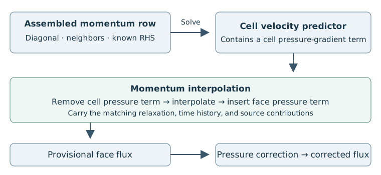
Fig. 5.3.2.1 The momentum row supplies a cell velocity. Momentum interpolation replaces its cell pressure-gradient term with a face pressure-difference term. Pressure correction then adjusts the face flux to satisfy continuity.#
For the classical gradient form,
Substitute this pressure contribution into the row and divide every term by \({}^{(u)}\!a_P\):
The second term is the pressure-gradient term in the cell velocity equation. Its coefficient, \(\Omega_P/{}^{(u)}\!a_P\), comes from dividing the momentum row by its diagonal. To see how this coefficient relates changes in the two quantities, hold \(\Omega_P\), \({}^{(u)}\!a_P\), and \(\vec H_P\) fixed. A change in the pressure gradient then gives
Here \(\Delta\) denotes a change. The pressure-gradient change is the input; the cell-velocity change is the output. This is the sensitivity of cell velocity to the pressure gradient for the fixed momentum row. The minus sign gives the direction of the velocity change, and \(\Omega_P/{}^{(u)}\!a_P\) sets its magnitude. We use this coefficient when constructing the pressure term at the face.
Define the momentum pseudovelocity as the nonpressure velocity contribution:
Rearrange Eq. (5.3.2.4) to evaluate it from the solved cell velocity:
We now have the pseudovelocity \(\hat{\vec u}_P\) and the coefficient \(\Omega_P/{}^{(u)}\!a_P\) multiplying the pressure gradient. The face construction uses both quantities from each adjacent cell.
5.3.3. Constructing the Flux on an Orthogonal Face#
To construct the face-normal velocity from the cell relation in Eq. (5.3.2.4), we need a face value of the pseudovelocity, a coefficient multiplying the pressure gradient, and an estimate of the face-normal pressure gradient.
For the face construction, label the left cell \(P\) and the right cell \(N\). Take an orthogonal face, whose cell-center line is parallel to its stored normal. First interpolate the nonpressure velocity from the two cells:
Interpolate the coefficient \(\Omega/{}^{(u)}\!a\) multiplying the pressure gradient using the same weights:
These interpolations supply the first two quantities. For the remaining quantity, the face-normal pressure gradient, use the pressure difference between the two cells. Let \(\vec x_P\) and \(\vec x_N\) be their center positions, with
The center spacing on this orthogonal face is
On this orthogonal face, \(\ell_f\) is also the center-to-center distance.
Approximate the face-normal pressure gradient by the pressure difference divided by that distance:
This gives the exact gradient for a linear pressure field. Equations (5.3.3.1), (5.3.3.2), and (5.3.3.5) now supply all three quantities. Using these three approximations in the face form of Eq. (5.3.2.4) gives
Multiply the normal velocity by the face area to obtain volume flow rate:
Substituting the reconstructed normal velocity defines the provisional flux:
5.3.4. Writing the Flux in Terms of Cell Velocities#
Equation (5.3.3.8) gives the provisional flux in terms of pseudovelocities. Substituting their definitions expresses the same flux using the solved cell velocities and identifies the momentum-interpolation correction. The two cell relations are
Substitute these expressions into the interpolated pseudovelocity term in Eq. (5.3.3.8) and collect the velocity and pressure terms:
The first term is the interpolated cell flux. The second adds back the cell pressure-gradient term, removing that term from the interpolated velocity. Substitute this expansion into Eq. (5.3.3.8):
Provisional Face Flux
This completes the construction outlined in Eq. (5.2.6). The first term interpolates the cell velocities; the remaining two terms form the momentum-interpolation correction.
Multiply the volume flux by the face density to obtain the mass flux:
5.3.5. A Compact Pressure-Difference Form#
Equation (5.3.4.3) contains two pressure terms: the positive term formed from the reconstructed cell gradients and the negative term formed from \(p_N-p_P\). We now combine them to express the correction as a difference between two estimates of the pressure change across the face.
To give these terms a common coefficient on the orthogonal face, interpolate the coefficient \(\Omega/{}^{(u)}\!a\) and the pressure gradient separately, then multiply the two interpolated quantities. This gives the product approximation:
Use \(\mathcal I_f(q)=w_Pq_P+w_Nq_N\) to write these interpolations more compactly. The center-to-center vector on this face is \(\vec r_{PN}=\ell_f\hat{\vec n}_f\). The component of the interpolated gradient normal to the face can therefore be written as
Apply the product approximation and substitute this geometric identity into the cell pressure term:
The two pressure terms now share a coefficient and denominator:
Factor out the common coefficient. The bracket compares the direct pressure change \(p_N-p_P\) with the change \(\mathcal I_f(\nabla p)\cdot\vec r_{PN}\) obtained from the cell gradients:
Substitute this combined pressure term into Eq. (5.3.4.3):
This is the compact form of the flux in Eq. (5.3.4.3), using the product approximation in Eq. (5.3.5.1). Its correction compares the adjacent-cell pressure difference with the pressure change obtained from the reconstructed cell gradients.
For a linear pressure field with exact reconstructed gradients, the two pressure changes agree and the correction is zero. For the alternating field in the checkerboard example, the cell gradients are zero, and the adjacent-cell pressure difference produces a nonzero face-flux correction.
The product approximation is the additional step that made this compact form possible. The difference between the original interpolated product and its approximation is
This approximation is exact when either the coefficient \(\Omega/{}^{(u)}\!a\) or the reconstructed pressure gradient is the same in both cells.
The classical Cartesian derivation develops the uniform-grid expression and its Taylor expansion, which describes the accuracy of the face interpolation for smooth pressure fields.
5.3.6. Geometry and the Two Pressure Reconstructions#
The preceding construction assumes that the cell-center line is parallel to the face normal. For a non-orthogonal face, we must account for their different directions when reconstructing the normal pressure gradient.
For a general face, use the transport chapter’s center-line geometry: \(d_{PN}=\lVert\vec r_{PN}\rVert\), \(\hat{\vec r}_{PN}=\vec r_{PN}/d_{PN}\), and \(\ell_f=\vec r_{PN}\cdot\hat{\vec n}_f>0\), with \(P\) and \(N\) in the stored left-to-right order. The angle between \(\hat{\vec r}_{PN}\) and \(\hat{\vec n}_f\) measures non-orthogonality. Face-center skewness is the displacement of the face centroid from the chosen interpolation point on the center line.
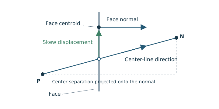
Fig. 5.3.6.1 Cell-center direction, face normal, and face-centroid displacement.#
Let \(\vec r_t=\vec r_{PN}-\ell_f\hat{\vec n}_f\) be the transverse part of the center-to-center vector. For a linear pressure field,
Divide by \(\ell_f\) and subtract the transverse term to obtain the normal pressure gradient. Using interpolated cell gradients for that term gives
The first term uses the adjacent-cell pressure difference. The second is the transverse correction, evaluated from lagged reconstructed cell gradients. Keeping only the first term gives the two-point reconstruction in Eq. (5.3.3.5) [FP02].
The normal derivative and the face pressure used in the cell momentum balance are different quantities. A transverse correction to the derivative does not correct a pressure value interpolated away from the face centroid. The latter requires a face-value reconstruction, developed below. In either construction, the two pressure derivatives subtracted in the MI term must be measured in the same direction.
The classical, Pascau and Choi derivations below use orthogonal face geometry. Their relaxation and time-history algebra does not specify a unique extension to nonorthogonal faces. Such an extension must state how both the cell and face pressure terms are projected. Denner’s construction in Denner Unified Momentum-Weighted Interpolation makes this choice explicitly by comparing both terms along the center line.
5.3.7. Face Pressure and the Cell Pressure Force#
The pressure term in the cell momentum balance approximates a surface integral. With one pressure value \(p_f\) per face, define the integrated pressure gradient as
Its contribution to momentum is \(-\vec{\mathcal P}_P\). A shared face pressure gives equal and opposite contributions to its two cells. The choice of \(p_f\) determines the accuracy of this force.
Central interpolation (pressureReconstruction=CD) uses
The ordinary CD weights use the distances from each cell center to the face: \(w_N=\lVert\vec x_f-\vec x_P\rVert/ (\lVert\vec x_f-\vec x_P\rVert+\lVert\vec x_N-\vec x_f\rVert)\). Denner instead uses the projected-distance weights in Eq. (5.8.1.5). In each case, these are the weights used in \(\mathcal I_f\) for the pressure reconstruction.
For a linear pressure field, central interpolation gives the exact pressure at \(w_P\vec x_P+w_N\vec x_N\). This point need not be the face centroid. Taylor expansion from that point to \(\vec x_f\) gives the corrected form
For a linear field with constant gradient,
\(w_Pp_P+w_Np_N=p(\vec x_f)-\nabla p\cdot\vec r_f\).
The added term therefore recovers \(p(\vec x_f)\) when the reconstructed
gradients are exact. Denner’s highOrder option uses this correction with
its CD weights.
The MUSCL pressure reconstruction first extrapolates from each neighboring cell and then averages the two face values:
Here \(\Psi\) is the gradient limiter used in the transport chapter.
The value \(\Psi=1\) leaves the gradient unchanged. With exact gradients and
\(\Psi_P=\Psi_N=1\), both extrapolations equal \(p(\vec x_f)\) for a linear
field. Unlimited MUSCL and corrected CD thus agree for that field, even
with unequal geometric weights. They generally differ for curved pressure
fields, approximate gradients or active limiting. Setting both MUSCL
limiters to zero gives the arithmetic mean of the cell pressures, which
equals distance-weighted CD only for equal weights or equal pressures.
The option pressureReconstruction=MUSCL selects this averaged pressure;
it is the default in momentumEquationOptions.
Substitute the selected \(p_f\) into Eq. (5.3.7.1) to obtain the cell pressure contribution. On a planar face, a linear pressure also satisfies
Thus exact reconstruction at the area centroid integrates a linear pressure exactly. Exact reconstruction at an arbitrary face point does not have this property. Curved pressure fields still incur quadrature error, and a nonplanar face requires its varying normal to be included in the surface integration. These spatial approximations affect the converged momentum balance, independent of how accurately the pressure-correction iteration is solved.
5.4. Classical Rhie–Chow Form and Under-Relaxation#
This section describes momentumInterpolationOptions: <form=old>, including
its Majumdar iteration-history term.
Iteration and Stage Notation
The superscript \(k\) identifies a completed outer, or Picard, iteration, while \(k+1\) identifies the iteration being advanced. A star identifies the provisional momentum-predictor stage before pressure correction, and a prime identifies the correction obtained from the pressure-correction equation. The basic algorithmic sequence is
A superscript \(n\) identifies a physical time level, independently of \(k\). When only the predictor stage matters, \(\vec u^*\) and \(\dot\Omega_f^*\) stand for \(\vec u^{*,k+1}\) and \(\dot\Omega_f^{*,k+1}\).
5.4.1. Relaxation of the Momentum Row#
Let \({}^{(u)}\!a_P\) and \({}^{(u)}\!\vec b_P\) denote the unrelaxed assembled row, and let \(0<\alpha_v\leq1\) be the velocity relaxation factor. Add \([(1-\alpha_v)/\alpha_v]{}^{(u)}\!a_P (\vec u_P^*-\vec u_P^k)\) to the left side of that row. This addition vanishes when the iteration stops changing. Moving its known \(\vec u_P^k\) term to the right gives
The diagonal is divided by \(\alpha_v\); the neighbor coefficients are unchanged. The last term is a known source that restores the original row when the iteration converges. In the algorithm chapter’s notation,
Dividing Eq. (5.4.1.1) by its diagonal, and collecting the nonpressure neighbor and source terms into \(\vec H_P\), gives the velocity relation below. Neighbor velocities inside \(\vec H_P\) are those of the implicit predictor solution, not a separately relaxed explicit update.
The resulting provisional cell velocity is
The bracket is the same momentum relation as Eq. (5.3.2.4), evaluated with the new predictor’s neighbor velocities. With \(\alpha_v=1\), the previous-iteration term disappears. With \(\alpha_v<1\), part of the previous corrected velocity is retained.
The volumetric flux obtained by interpolating the previous cell velocities is
This interpolation generally differs from the stored face flux \(\dot{\Omega}_f^{\,k}\). Their difference is
The difference is already known from iteration \(k\). It contains the face-specific contribution that is not reproduced by simply interpolating the cell velocities. Majumdar’s construction carries the fraction \(1-\alpha_v\) of this previous face-flux difference into the new provisional flux [Maj88].
The new predictor already contains the interpolated part of the previous
cell velocity. Carry the remaining previous face-flux difference separately.
Combining it with the two pressure terms gives the expanded form=old result:
Each coefficient \(\Omega/{}^{(u)}\!a\) uses the complete unrelaxed diagonal. Integrated pressure and body-source replacements are developed in Consistency with Momentum Source Terms.
At convergence, the predictor and corrected quantities agree between iterations. Denote the remaining difference between the face flux and the interpolated cell flux by
Subtract the interpolated velocity term from Eq. (5.4.1.6). The same difference now occurs on both sides:
Move the last term to the left. Its coefficient becomes \(1-(1-\alpha_v)=\alpha_v\). Dividing by \(\alpha_v>0\) leaves
This is the unrelaxed pressure contribution. The previous face-flux difference is therefore what removes the explicit relaxation factor from the converged relation. Its temporal dependence is addressed next.
We now combine the two pressure terms in the expanded flux, Eq. (5.4.1.6), using the steps from A Compact Pressure-Difference Form. Interpolate the coefficient and pressure gradient separately, then multiply them. Use the interpolated gradient to estimate the pressure change between cell centers. These substitutions give the compact flux formula:
The history term is unchanged. The pressure terms carry the additional approximations used to obtain the compact form.
Let \(\vec x_f\) be the face-center position. For this family, the interpolation weights are based on the cell-center-to-face distances:
5.4.2. Relaxing Only the Spatial Diagonal#
An alternative is to relax only the non-temporal part of the row. Write \(\widetilde a_P={}^{(u)}\!a_{P,\mathrm{spatial}}\) and let \(T_P={}^{(u)}\!a_{P,\mathrm{time}}\). Whole-diagonal relaxation and spatial-only relaxation then give, respectively,
The deferred relaxation source is respectively
\((1-\alpha_v)(\widetilde a_P+T_P)\vec u_P^k/\alpha_v\) or
\((1-\alpha_v)\widetilde a_P\vec u_P^k/\alpha_v\).
Their different predictor diagonals give different coefficients multiplying
the pressure gradient in the velocity equation at finite iteration. The
derivations here use whole-diagonal relaxation. Spatial-only relaxation is
an algebraic alternative, not another form selector in the table above.
5.5. Time-Consistent Momentum Interpolation#
The Pascau construction in this section corresponds to
momentumInterpolationOptions: <form=new>. The complete one-step derivation
uses a fixed grid and the continuity-subtracted BDF1 momentum row. Time-step
independence below refers to the converged steady limit; transient solutions
still have the truncation error of their time discretization.
The classical momentum-interpolation construction uses the assembled momentum diagonal in the coefficient multiplying the cell pressure gradient. In a transient calculation, that diagonal contains a contribution from the time derivative as well as contributions from convection, diffusion, and any other terms treated implicitly. The temporal contribution can be seen directly from the discretized momentum storage term.
For a representative BDF1 step, after the continuity-consistent velocity form has been obtained and with \(\rho_P\Omega_P\) evaluated at the previous physical time level, the temporal contribution is
The current physical-time index on \(\vec{u}_P^{*,k+1}\) is suppressed; the star and \(k+1\) identify the momentum predictor within that time step. When the momentum row is assembled, the coefficient multiplying \(\vec{u}_P^{*,k+1}\) is placed on the left-hand side. The known term containing \(\vec{u}_P^n\) is moved to the right-hand side. Thus BDF1 adds \(\rho_P^n\Omega_P^n/\Delta t\) to the diagonal of every velocity-component row.
Within this continuity-subtracted temporal split, let \(\lambda_0\) denote the coefficient of the current-time contribution retained implicitly. BDF1 has \(\lambda_0=1/\Delta t\); the multistep split is developed below. The complete momentum diagonal is then
The shorthand \(\widetilde a_P={}^{(u)}\!a_{P,\mathrm{spatial}}\) is what remains after the current-time temporal contribution is removed. It contains the convective, diffusive, and other non-temporal contributions treated implicitly in the momentum row.
The temporal coefficient in this split belongs to the stated momentum-row form. It is not a universal replacement for the conservative or multistep temporal diagonal. Also, \(\widetilde a_N\) is the non-temporal diagonal of cell \(N\), not the coupling \({}^{(u)}\!a_{P,N}\) in the row for \(P\).
Using the complete \({}^{(u)}\!a_P\) in the classical coefficient \(\Omega_P/{}^{(u)}\!a_P\) introduces a temporal contribution into the face interpolation. The coefficient depends on the time step:
For BDF1, reducing \(\Delta t\) increases \(\lambda_0=1/\Delta t\) and therefore reduces \(\Omega_P/{}^{(u)}\!a_P\) when the other quantities are held fixed. If no matching face-flux history is carried, a converged nominally steady result can retain a residual dependence on the time step used to reach it. Time-consistent formulations use \(\Omega_P/\widetilde a_P\) and carry the corresponding physical-time history at the same face location as the new flux [Cho99, Pas11].
The ratio of the temporal diagonal to the non-temporal diagonal is
For BDF1, this becomes \(\delta_P=(\rho_P^n\Omega_P^n/\Delta t)/\widetilde a_P\). The ratio therefore measures the temporal contribution to the diagonal relative to the non-temporal contribution. The complete diagonal can be written
For the face shared by cells \(P\) and \(N\), the same geometric weights used in the momentum interpolation give
5.5.1. Deriving the Complete One-Step Face Relation#
The nonpressure group \(\vec H_P\) contains the old-time momentum as well as the spatial terms. Expose those two pieces before dividing the row:
Divide the spatial group by \(\widetilde a_P\) and call the resulting velocity \(\vec h_P\):
Thus \(\vec H_P=\widetilde a_P\vec h_P+ {}^{(u)}\!a_{P,\mathrm{time}}\vec u_P^n\). Substitute this and \({}^{(u)}\!a_P=\widetilde a_P+{}^{(u)}\!a_{P,\mathrm{time}}\) into the relaxed momentum row:
Multiply by \(\alpha_v/\widetilde a_P\). The two ratios that appear are
Replacing these ratios by their names gives
For the face, interpolate \(\vec h\), \(\delta\), and \(\Omega/\widetilde a\) with the selected geometric weights. Use the face’s own old-time and old-iteration fluxes in its history terms. The analogous face relation is defined by
This is an interpolation model for the face, not a new equation solved on a face control volume. Eliminate \(\mathcal I_f(\vec h)\) using the two cell rows. Rearranging and interpolating Eq. (5.5.1.5) gives
The ratios remain inside the interpolation of each cell velocity. For example, the provisional-velocity term expands as
It reduces to ordinary interpolation if \(\delta_P=\delta_N\). For unequal ratios, each cell velocity retains its own multiplier.
Now multiply Eq. (5.5.1.7) by \(A_f\), project onto the face normal, and substitute it into the face relation. Collect terms from the same time or iteration level:
The positive history terms came from the face relation. The negative ones came from eliminating the cell quantity \(\vec h\). Their subtraction replaces the history already carried by the cell velocities with the face’s own history.
5.5.2. Face-Flux History Terms#
Call the last bracket \(\eta_f^n\), the weighted difference between the previous-time face flux and the flux represented by the cell velocities:
Call the previous-iteration bracket \(\eta_f^k\):
After division by \(1+\delta_f\), the two history groups contribute
The cell and face histories are therefore treated as one discrete temporal system. With these definitions, the full one-step result is
Complete Pascau Construction
The four terms are the weighted provisional velocity, removal of the cell pressure-gradient term, insertion of the face pressure-difference term, and matched iteration/time history. Changing only the pressure coefficient does not produce this construction. A conservative pressure replacement changes the cell pressure term as described in Consistency with Momentum Source Terms.
5.5.3. Reading the Pressure Coefficient from the Flux#
In the completed face formula, hold the predictor, histories, gradients, and coefficients fixed. Only the direct pressure-difference term changes when \(p_N-p_P\) changes. Multiply its volume-flux coefficient by \(\rho_f\) to obtain the direct mass-flux coefficient \(d_f^{\mathrm{dir}}\). The signed sensitivity of face mass flux to \(p_N-p_P\) is \(-d_f^{\mathrm{dir}}\); increasing that pressure difference decreases the flux in the stored direction.
The classical old selection uses the complete momentum diagonal in
its direct pressure coefficient, while the one-step time-consistent
new selection uses the non-temporal diagonal together with
\(1+\delta_f\):
The superscript \(\mathrm{dir}\) identifies the direct pressure-difference
term. The coefficient \(d_f\) used in the pressure-correction equation may
also include a stated approximation to the cell-velocity change, as derived
in Connection to the Pressure-Correction Equation.
The superscripts \(\mathrm{old}\) and \(\mathrm{new}\) identify the Stream
momentum-interpolation selections; they are not physical-time levels. Both
expressions give the magnitude of the face mass-flux sensitivity to the
adjacent-cell pressure difference, with the remaining predictor quantities
held fixed. The new coefficient makes two changes: it uses the non-temporal
cell ratios \(\Omega/\widetilde a\), and it divides the resulting face
coefficient by \(1+\delta_f\).
5.5.4. Checking the Steady Limit#
To check the steady limit, define the spatial pressure contribution
At a converged steady state, the old-time, old-iteration, and provisional velocities all equal \(\vec u\), and the corresponding face fluxes equal \(\dot\Omega_f\). Insert these equalities into the expanded substitution. Move the history terms containing face flux to the left, and collect the cell-velocity terms on the right:
Both brackets reduce to \(\alpha_v\), even when the two cell ratios differ. Dividing by \(\alpha_v>0\) gives
Neither the temporal ratio nor the relaxation factor remains in this steady-limit relation. This cancellation uses the weighted predictor as well as both history terms; the history terms alone do not vanish separately for unequal cell ratios.
5.5.5. Multistep and Crank–Nicolson Extensions#
For constant step and fixed cell mass \(M_P=\rho_P\Omega_P\), start with the usual BDF2 storage term. Regroup its three velocity values as two increments:
The first current-velocity term is implicit; the second current-velocity term is lagged during assembly. At convergence this is the usual BDF2 derivative. It gives \(\delta_P=2M_P/(\Delta t\widetilde a_P)\) and \(\epsilon_P=M_P/(2\Delta t\widetilde a_P)\). The fully implicit BDF2 diagonal \(3M_P/(2\Delta t)\) must not be substituted for the leading split diagonal while retaining these history terms.
In the face construction, the older increment contributes a current-velocity term as well as an old-time term. Collecting the current terms gives the face multiplier
Here \(\epsilon_f=\mathcal I_f(\epsilon)\) uses the older-history coefficient just defined; it is not a stored value of \(\delta\).
With \(\Xi_P=1+\delta_P-\alpha_v\epsilon_P\) and \(\Xi_f=\mathcal I_f(\Xi)\), the corresponding assembled face result is
The definitions of \(\eta_f^k\) and \(\eta_f^n\) retain the current \(\delta\) coefficients. The face construction evaluates the split current-level contribution with the predictor velocity; the cell momentum assembly may lag that contribution during its solve. This additional face choice agrees with the cell split at outer-iteration convergence. This formula displays all three changes from BDF1: the predictor weighting, denominator, and older-history difference. For variable steps, with \(h=\Delta t_n\) and \(k_t=\Delta t_{n-1}\), the corresponding split coefficients are
Each history carries its own mass. Subtracting the two current-level coefficients recovers the usual leading BDF2 coefficient at constant mass. The variable-step derivative and continuity subtraction are developed in (10.3.2.6) and (10.3.3.1). The time-step symbol \(k_t\) here is unrelated to the outer-iteration index \(k\).
Crank–Nicolson can be normalized by dividing its half-weighted current spatial residual by \(1/2\). The temporal coefficient is then \(2M_P/\Delta t\) and the known old spatial residual also enters the RHS. This has the one-step face-history structure above with its correctly assembled \(\widetilde a_P\) and \(\delta_P\); it has no \(n-1\) history. In particular, \(\Delta t\delta_P/\rho_P=2\Omega_P/\widetilde a_P\) in this normalization. Replacing \(\Omega/\widetilde a\) by \(\Delta t\delta/\rho\) without that factor of two would change the coefficients multiplying the pressure terms. See (10.3.2.11) for the temporal normalization.
5.6. Choi-Style Face History#
The selection momentumInterpolationOptions: <form=Choi> retains the
classical relaxed flux and adds a previous-time face–cell flux difference.
The variant developed here uses one common temporal ratio at the face.
This averaging choice is part of the formulation; it is not an exact
rearrangement of cell-specific temporal weights.
5.6.1. Constructing the History Weight#
For BDF1 at fixed cell mass, the fraction of the unrelaxed momentum diagonal supplied by storage is
The previous cell velocity therefore contributes \(\alpha_v\delta_P\vec u_P^n/(1+\delta_P)\) to the relaxed predictor. The Choi variant uses the interpolated ratio \(\delta_f=\mathcal I_f(\delta)\) to weight an additional history term:
The same face coefficient multiplies both stored quantities in the bracket. The predictor still contains its cell-specific history weights. Combining that contribution with the added correction gives
When \(\delta_P=\delta_N\), the last term vanishes, leaving only the weighted previous face flux. For unequal ratios, part of the cell history generally remains. The added term therefore replaces the full interpolated cell history only when the weights agree or the remaining term happens to cancel for the particular velocity field.
Adding \(\mathcal C_{f,\mathrm{Choi}}\) to Eq. (5.4.1.6) gives the complete one-step formula, with momentum sources omitted:
The direct pressure coefficient is unchanged from old. The predictor and cell-pressure term still use the complete cell diagonal. Pascau instead retains the cell-specific temporal ratios in both its weighted predictor and histories, as derived in Time-Consistent Momentum Interpolation.
5.6.2. Steady Limit of the Choi Form#
At a converged steady state, both stored face–cell flux differences equal \(E_f=\dot\Omega_f-\mathcal I_f(\vec u)\cdot\vec A_f\). Move those history terms to the left of Eq. (5.6.1.4):
Divide by \(\alpha_v/(1+\delta_f)\) and substitute \({}^{(u)}\!a=\widetilde a(1+\delta)\):
For equal temporal ratios, the ratio inside each interpolation is one, and the result is the spatial pressure contribution \(\mathcal C_{p,f}\) of Eq. (5.5.4.1). For unequal ratios, those factors generally retain timestep dependence. The explicit relaxation factor cancels in either case. Pascau’s steady cancellation holds for unequal ratios as well, because its predictor and both histories carry the matching cell-specific weights.
5.7. Consistency with Momentum Source Terms#
Equation (5.3.2.3) represents the integrated pressure gradient as \(\Omega_P\nabla p_P\). A momentum balance using the face-pressure sum in Eq. (5.3.7.1) instead contains \(\vec{\mathcal P}_P\). A gradient reconstructed independently need not satisfy \(\Omega_P\nabla p_P=\vec{\mathcal P}_P\). Removing a different pressure contribution from the cell velocity introduces a discrepancy between the cell momentum balance and the face construction.
Use the same integrated pressure gradient when separating the cell velocity:
Interpolate \(\vec{\mathcal{P}}_P/{}^{(u)}\!a_P\) when removing the pressure contribution already contained in the cell velocities. The same principle applies to a discrete body-force source \(\vec{\mathcal{B}}_P\).
The conservativePressure modifier selects this integrated pressure
contribution for old, new, and Choi, while retaining their direct
adjacent-cell pressure difference. Denner uses the integrated contribution
as part of its formulation.
For a stationary state with no remaining momentum terms,
the face-pressure and body-force corrections should cancel when their direct face reconstructions also satisfy the corresponding balance. This requires compatible interpolation and geometry at both locations. A mismatch can generate a nonzero face flux even when the cell momentum residual is zero. This condition applies to hydrostatic, rotating-frame, and other stationary source-balanced solutions.
Discrete Compatibility Condition
Preserving an equilibrium requires both cancellation of the integrated cell forces and compatible direct pressure/source reconstructions at the face. Cell cancellation alone is insufficient. These are discrete balance conditions, beyond agreement in the continuum limit.
5.7.1. Removing and Replacing a Source Contribution#
First consider a body force supplied explicitly to the momentum equation. Let \(\vec S_P\) be this force per unit volume, and let \(\vec{\mathcal B}_P\) be its integrated contribution to the cell momentum row. In the divided Pascau row, this source contributes
Therefore the weighted predictor in the face formula already carries \(\alpha_v A_f\mathcal I_f(\vec{\mathcal B}/\widetilde a) \cdot\hat{\vec n}_f\). A separate face source must replace this contribution.
To construct that face source, start with the pressure change needed to balance it. Integrate along the two segments from \(P\) to the face center and from the face center to \(N\). With a constant source on each segment,
The line estimate \(L_f(\vec S)\) has pressure units. Dividing by \(\ell_f\) gives the direct face source used in the normal-velocity relation. The Pascau flux therefore needs the following change:
Call this pair \(\mathcal C_{S,f}(1+\delta_f)\). Other formulations use the same removal and replacement with a different face denominator. Writing that denominator as \(\Xi_f\) gives the reusable expression
For Pascau, \(\Xi_f=1+\delta_f\). For the classical formulation, replace \(\widetilde a\) by the complete diagonal and use \(\Xi_f=1\).
The pressure contribution with integrated cell pressure is
Add the pressure and source corrections and collect their cell and face terms separately:
The first line vanishes when the integrated forces balance in each cell. The second vanishes when the adjacent pressure difference equals the source line estimate. Both are required to preserve the equilibrium. For a velocity-dependent force, the face correction must be specified together with the source linearization. In the porous construction, the positive implicit resistance remains in the momentum diagonal, while the pressure–source correction uses the complete physical force. The linearization remainder defines the momentum RHS; it is distinct from the force used in that face balance. Equation (19.4.1) gives the porous correction and Eq. (19.4.2) shows its cancellation with pressure.
5.8. Denner Unified Momentum-Weighted Interpolation#
This section describes momentumInterpolationOptions: <form=Denner>.
The Bartholomew–Denner construction uses the same basic operation as the
preceding sections: remove the pressure and source contributions carried by
the cell velocities and insert their direct face counterparts. Its distinct
choices concern the shared face coefficient, density weighting, and face
history [BDAA+18].
The derivation below uses BDF1, a fixed grid, the continuity-subtracted
momentum row, and central interpolation of pressure for the cell force.
The pressure reconstruction is a separate choice in Stream: selecting
form=Denner selects its source weighting, but does not select central
pressure interpolation. The ordinary MUSCL pressure reconstruction remains
the default. Its cell force can be used in the face-pressure difference
below, but the central-interpolation equilibrium argument then needs to be
re-examined. The three reconstruction choices are distinguished in
Geometry and Source Modifiers.
5.8.2. Removing Cell Pressure and Sources, Then Inserting Face Values#
For pressure, the direct face value is \((p_N-p_P)/d_{PN}\). The cell value is obtained from the integrated pressure gradients, divided by cell mass, interpolated, and multiplied by \(\rho_{h,f}^k\). Their difference is
Thus \(-\mathcal D_f A_f\mathscr R_{p,f}\) adds back the pressure term represented by the cells and subtracts the face pressure-difference term, with the same signs as in the classical construction.
For a body source, the cell contribution enters velocity with a positive sign. Its replacement therefore has the opposite order: remove the cell contribution and add the direct face source. Define
Both differences have pressure-gradient units. Their combined spatial contribution to volume flux is \(\mathcal D_f A_f(-\mathscr R_{p,f}+\mathscr R_{b,f})\). The term residual here means a difference between two reconstructions; it is not the residual of a separate equation solved on the face.
For the gravity source, the direct face estimate uses the complementary weights
Their role follows from the source line estimate. On an orthogonal face, let \(h_P\) and \(h_N\) be the distances from each center to the face. Then \(w_N=h_P/d_{PN}\) and \(w_P=h_N/d_{PN}\), giving
The velocity weights would exchange the two segment lengths in this source estimate. For gravity with a consistently subtracted reference density, \(\vec S_P=(\rho_P-\rho_{\mathrm{ref}})\vec g\).
The integrated cell forces must use the matching reconstruction. With \(p_f=w_Pp_P+w_Np_N\), the pressure-gradient contribution is \(\vec{\mathcal P}_P=\sum_{f\in\mathcal F_P}\sigma_{Pf}p_f\vec A_f\). The corresponding interior-face additions to the body source are
Both expressions use the same stored area vector. Reversing the center line and area together leaves the physical source unchanged. At a physical boundary, the one-sided addition is \([\vec S_P\cdot(\vec x_f-\vec x_P)]\vec A_f\) for the physical owner. These source contributions are the ones removed in Eq. (5.8.2.2).
For a closed cell, \(\sum_f\sigma_{Pf}\vec A_f=\vec0\). Subtracting \(p_P\sum_f\sigma_{Pf}\vec A_f\) from the central pressure sum expresses it in terms of pressure differences. For a cell whose faces are all interior, with neighbor \(N\) across each face,
Here \(w_N\) is the weight of the neighboring cell in the face pressure, and \(\vec r_{PN}\) points from \(P\) to that neighbor; the incidence sign converts the stored area to the outward area of \(P\). Boundary rows use the corresponding one-sided pressure and source estimates. If \(p_N-p_P=\vec S_f\cdot\vec r_{PN}\) on every interior face, the cell sums agree. The direct face estimates then agree as well, so \(\mathscr R_{p,f}=\mathscr R_{b,f}\) and their flux contributions cancel. The skew correction below extends this pairing to corrected central pressure.
5.8.3. Including Face Time History#
First take \(\alpha_v=1\). As in the classical derivation, separate the face flux from the flux represented by the cell velocities. Write the current difference as \(E_f\) and the stored differences as \(E_f^j\):
Using the shared face coefficient, the face time coefficient is \(c_f=\rho_{h,f}^n\lambda_0\). Subtracting the interpolated cell storage increment from the face storage increment gives
Storage is on the left of the momentum balance, so its contribution on the source side is \(-c_f(E_f-E_f^n)\). Combine it with the pressure and body-source differences. Let \(\beta_f\) be the common geometric multiplier on those two spatial terms; the default is \(\beta_f=1\), and the optional angular corrections are given below. The resulting face model is
The choice of a shared face coefficient and harmonic density enters in forming this model. The next steps are algebra. Move the term containing the unknown current difference to the left:
Divide by \(1+c_f\mathcal D_f\) and label the two resulting factors:
Thus the coefficient multiplying the pressure and source terms is \(F_f\), and the old-time weight is \(G_f\):
For under-relaxation, retain the fraction \(1-\alpha_v\) of the previous iteration’s flux difference and use \(\alpha_v\) of the new difference just derived. This is the same face-history construction used for the classical form:
Add back the interpolated predictor and expand the two stored differences:
For equal density, equal cell ratios \(\Omega/\widetilde a\), midpoint weights, and an orthogonal face, \(c_f\mathcal D_f=\delta_f\). The Denner and Pascau history and pressure factors then coincide. Equal spacing alone is insufficient when density or the ratio \(\Omega/\widetilde a\) differs between the cells.
At a converged steady state, all three face–cell flux differences coincide. Subtract the iteration-history term and divide by \(\alpha_v\) to get \((1-G_f)E_f=\beta_f F_f A_f(-\mathscr R_{p,f}+\mathscr R_{b,f})\). Since \(1-G_f=1/(1+c_f\mathcal D_f)\), the ratio \(F_f/(1-G_f)=\mathcal D_f\). The complete steady flux difference therefore uses the spatial coefficient \(\mathcal D_f\), with no remaining temporal factor.
5.8.4. Geometry and Source Modifiers#
The factor \(\beta_f\) scales the pressure and source terms in the face flux
when the center line and normal are not parallel. The setting skewnessCorrection=1 uses \(\beta_f=1\);
this is also the default. The choices skewnessCorrection=2 and
skewnessCorrection=3 use, respectively,
These factors depend on the angle between the face normal and the center line. All three coincide on an orthogonal face. The third changes \(A_f/d_{PN}\) into \(A_f/\ell_f\); the same factor multiplies both pressure and source residuals.
With central pressure interpolation and highOrder, use the corrected
face pressure in Eq. (5.3.7.3) with the
projected-distance weights in Eq. (5.8.1.5). This changes
the integrated cell pressure contribution while retaining the direct
adjacent-cell pressure difference.
The published force-balanced construction includes the same interpolation correction in the cell source (Bartholomew et al., Eqs. 72–73 [BDAA+18]). Define its integrated face contribution as
The corresponding interior-face source additions are
The pressure-gradient sum gains \(+\vec k_f\) in the left cell and \(-\vec k_f\) in the right cell. Each source addition gains the same term, so the correction cancels from \(-\vec{\mathcal P}+\vec{\mathcal B}\). This preserves the central pressure/source pairing. It does not establish that either reconstructed force is individually accurate away from equilibrium; the spatial accuracy of both forces remains a separate requirement. Because \(\vec k_f\) depends on pressure, its change also belongs in the pressure-correction derivation for this source construction.
Stream’s highOrder option applies Eq. (5.3.7.3)
to pressure, but does not supply the matching cell-source addition in
Eq. (5.8.4.3).
For the current Stream variants, the pressure choices are:
Cell pressure reconstruction |
Effect on the Denner construction |
|---|---|
CD |
Eq. (5.3.7.2) with projected-distance weights; the pairing in Eq. (5.8.2.6) applies. |
CD with |
Eq. (5.3.7.3); the published balance additionally requires Eq. (5.8.4.3). |
MUSCL |
Eq. (5.3.7.4); |
MUSCL’s agreement with corrected CD for an unlimited linear field does not extend this balance proof to arbitrary pressures or limiter values. Changing the gradient estimate or limiter changes the force reconstructed in the cells and therefore the pressure term removed in the face flux.
The pressure reconstruction and the interpolation of velocity to the face
are also distinct. Bartholomew et al., Section 3.1, permit a velocity-gradient
correction for the displacement between the interpolation point and face
centroid, but make this correction optional
[BDAA+18]. Stream’s Denner predictor and stored
velocity histories use the linear interpolation shown in
Eq. (5.8.3.8). The pressure highOrder modifier
does not add that velocity correction.
The modified source estimate is a Stream variant. Its direct gravity/source estimate uses
\(L_f(\vec S)/d_{PN}\) in place of \(\vec S_f\cdot\hat{\vec r}_{PN}\).
The integrated cell source additions in Eq.
(5.8.2.5) replace
\(\vec S_f\cdot\vec r_{PN}\) by \(L_f(\vec S)\) at the same time.
The pressure and cell-source removal remain projected along the center line.
Both the direct source and the cell source must be changed together.
5.8.5. Direct Interior Pressure Coefficient#
Hold the cell velocities, reconstructed forces, histories and coefficients fixed. Varying only the direct face-pressure difference gives
The one-sided boundary construction is developed with the pressure-correction boundary conditions.
5.9. Connection to the Pressure-Correction Equation#
Changing pressure changes the cell velocity, the cell pressure contribution, and the direct face-pressure term. We add these three changes to obtain the flux correction for each form. SIMPLE and SIMPLEC supply the cell-velocity approximation; a further face approximation can restrict the pressure coupling to the two cells beside the face.
Assumptions for the face correction
Use an orthogonal, unskewed face on a fixed mesh, BDF1, and density fixed over the step. Hold the momentum coefficients, pressure-reconstruction weights, gradient-operator coefficients, limiter values and stored histories fixed during the correction. Body sources are pressure-independent in the following cell and face formulas. Relaxation applies to the complete momentum diagonal. Denner has \(\beta_f=1\), and its current and old-time harmonic densities agree.
5.9.1. Direct Pressure-Difference Coefficient#
Hold the predictor, cell forces, histories, density and momentum coefficients fixed. Varying only \(p_N-p_P\) defines
A positive \(d_f^{\mathrm{dir}}\) means that increasing \(p_N-p_P\) reduces mass flux in the stored direction. Its value is given by Eqs. (5.5.3.1) and (5.8.5.1) for the preceding forms, with Choi using the old coefficient. This derivative includes only the direct face term.
5.9.2. The Four Face Formulas#
For old, Choi and new, use the integrated pressure contribution introduced in Consistency with Momentum Source Terms. If the face formula instead uses \(\Omega\nabla p\), the cancellation below requires that quantity to equal the pressure contribution used in the cell correction.
Denote the predictor interpolation by \(\mathcal U_f(\vec u)\) and the velocity contribution of an integrated cell force \(\vec X\) by \(\mathcal L_f(\vec X)\). The original face formulas give
Form |
Predictor interpolation \(\mathcal U_f(\vec u)\) |
Cell-force contribution \(\mathcal L_f(\vec X)\) |
|---|---|---|
|
\(\mathcal I_f(\vec u)\) |
\(\alpha_v\mathcal I_f(\vec X/{}^{(u)}\!a)\) |
|
\(\mathcal I_f[(1+\delta)\vec u]/(1+\delta_f)\) |
\(\alpha_v\mathcal I_f(\vec X/\widetilde a)/(1+\delta_f)\) |
|
\(\mathcal I_f(\vec u)\) |
\(\alpha_v\rho_{h,f}F_f\mathcal I_f(\vec X/M)\) |
Let \(\mathcal C_{f,\mathrm{hist}}\) denote the selected form’s total history contribution. It is the iteration term in Eq. (5.4.1.6) for old, the two history terms in Eq. (5.6.1.4) for Choi, Eq. (5.5.2.3) for new, and the two history terms in Eq. (5.8.3.8) for Denner. With momentum sources omitted, the four flux formulas can be written as
Here \(d_f^{\mathrm{dir}}\) is the original coefficient for the selected form. Fixed body-source terms may be included; they contribute no change during the pressure correction.
5.9.3. Correcting the Cell Pressure Contribution#
Following the pressure–velocity algorithms chapter, use the raw pressure correction in the trial fields:
The later primary-pressure update may be relaxed. The velocity and flux corrections use the raw \(p'\) from the pressure equation.
Apply the pressure correction to the face pressure used in the momentum equation. The integrated change is
For CD with fixed weights, \(p_f'=w_Pp_P'+w_Np_N'\). The corrected CD expression in Eq. (5.3.7.3) gives
For MUSCL, apply the same substitution to Eq. (5.3.7.4), holding \(\Psi_P\) and \(\Psi_N\) fixed:
Here \(\nabla p'\) is computed by the same linear gradient operator as \(\nabla p\). These expressions give the exact change for the frozen reconstruction. A full linearization of an active limiter would also include its change with pressure. Omitting the gradient terms is a further approximation, beyond freezing the limiter. The omitted changes must then be recovered by updating the reconstruction in the outer iteration; this does not guarantee that the iteration converges.
Subtract the predictor momentum row from the trial corrected row:
SIMPLE omits the neighboring velocity corrections, giving the approximate cell row
For SIMPLEC, rewrite the neighbor sum in Eq. (5.9.3.5) as a part proportional to \(\vec u_P'\) and a part containing differences:
This rearrangement is exact with the momentum coefficients held fixed. SIMPLEC neglects the weighted differences on the right, giving
Solving the two approximate rows gives the cell corrections, with the coefficients \(D_P\) used in the algorithms chapter:
The SIMPLEC denominator must be nonzero. A positive denominator gives a velocity change opposite to the pressure-gradient change. Its value must come from the assembled momentum row, including implicit sources and boundary contributions.
Both expressions use \(\vec{\mathcal P}_P'\) from the momentum pressure reconstruction. An algorithm may approximate this change with a simpler pressure-correction gradient. That adds an approximation; the exact cancellations below then hold only where the two operators agree.
5.9.4. Adding the Three Face-Flux Changes#
Hold the stored time and iteration histories and any body-source terms fixed. Evaluate Eq. (5.9.2.1) at the trial corrected fields and subtract its predictor value. Linearity of \(\mathcal U_f\) and \(\mathcal L_f\) gives
This expression gives the change in face flux for either cell correction under the stated assumptions.
5.9.5. Classical, Choi and Pascau Corrections#
With SIMPLE, \(\vec u_P'=-\alpha_v\vec{\mathcal P}_P'/{}^{(u)}\!a_P\). For old and Choi, ordinary interpolation makes the first two terms cancel. For new, substitute \({}^{(u)}\!a=\widetilde a(1+\delta)\):
These three forms therefore leave only the direct face-pressure term, provided the cell correction and the force removal use the same pressure reconstruction.
For an interior momentum row with no implicit sources or boundary contributions, the continuity-subtracted form gives \(\sum_N{}^{(u)}\!a_{P,N}=\widetilde a_P\). Since \({}^{(u)}\!a_P^{\mathrm{pred}}=\widetilde a_P(1+\delta_P)/\alpha_v\), the SIMPLEC cell coefficient exceeds the SIMPLE coefficient by the factor
Here
For old, Choi and new, the part equal to the SIMPLE correction still cancels the cell-pressure term. The additional part gives
To obtain a correction using only \(p_P'\) and \(p_N'\), make two face approximations. First, replace the cell-dependent multipliers by one face value, evaluated from \(\delta_f=\mathcal I_f(\delta)\):
Evaluating this ratio after averaging \(\delta\) generally differs from averaging the cell values of \(\kappa\). Second, replace the interpolated cell-pressure term by the adjacent-cell pressure difference:
Substituting these two approximations into Eq. (5.9.5.4) gives
The compact coefficient therefore uses both the SIMPLEC cell approximation and the two face approximations above. Implicit sources or other momentum-row forms change the neighbor-coefficient sum used to derive \(D_P^{\mathrm C}\).
5.9.6. Denner with SIMPLE and SIMPLEC#
Denner interpolates the predictor normally but weights the cell force with a shared, density-dependent coefficient. Substitution of the SIMPLE cell correction leaves
The remaining cell term vanishes when the two coefficients agree in each cell. Otherwise, \(\vec{\mathcal P}'\) brings in pressure corrections from the other faces of those cells.
For SIMPLEC, substitute \(\vec u_P'=-(D_P^{\mathrm C}/\Omega_P)\vec{\mathcal P}_P'\) into Eq. (5.9.4.1) and combine the two cell terms under the same interpolation:
The remaining cell term vanishes for arbitrary pressure corrections if its coefficient vanishes in each cell:
One shared face coefficient generally cannot satisfy these two cell conditions. The remainder may cancel for a particular pressure field without these coefficient equalities, but that is not a general identity.
Using \((1+\kappa_f)d_f^{\mathrm{dir}}\) as a compact coefficient for Denner requires an approximation to the entire remaining cell term in Eq. (5.9.6.2). The SIMPLEC cell approximation alone does not supply that face approximation.
5.9.7. Summary of the Pressure Corrections#
For the stated fixed-density, orthogonal scope, the cell contribution that remains after the direct term is
5.9.8. Using the Selected Correction in Continuity#
When the cell terms cancel, \(d_f=d_f^{\mathrm{dir}}\). When their effect is approximated by a two-cell pressure difference, include that approximation in \(d_f\), as in Eq. (5.9.5.7). The selected compact correction is then
If the cell terms are retained instead, multiply Eq. (5.9.4.1) by \(\rho_f\):
Insert the selected face correction into fixed-density continuity:
The pressure-correction chapter assembles the cell row and develops density corrections and boundary conditions. The pressure matrix and the applied flux correction must use the same face relation. Retaining the cell terms adds their pressure couplings; omitted changes remain to be resolved by the outer iteration.
For nonorthogonal faces, changes in transverse and skew corrections may be included or deferred to the outer iteration. A pressure-dependent body force contributes an additional change, as in the published corrected source construction in Eq. (5.8.4.3).
5.10. Moving Grids and Relative Flux#
On a moving control volume, continuity uses the fluid flux relative to the grid:
where \(\dot{\Omega}_{g,f}\) is the swept grid-volume flux. Momentum interpolation constructs the fluid flux and its dependence on the adjacent-cell pressure difference. Continuity and its flux correction use the relative flux. At the predictor stage, the relative flux supplied to the pressure-correction equation is therefore
The geometric conservation law also requires the same time-consistent face area representation in:
the transported face flux,
the pressure and source terms in the momentum-interpolation formula, and
the swept grid-volume flux.
Otherwise a uniform flow may acquire a nonzero discrete residual solely from mesh motion. The space–time area construction used for this purpose is developed in Geometric Conservation Law for Moving Meshes.
5.11. Comparing the Completed Constructions#
The fixed-grid, one-step forms combine the following momentum weights and histories, with the stated assumptions on spatial reconstruction.
Selection |
Momentum weighting |
History treatment |
Reconstruction assumptions |
|---|---|---|---|
|
Complete diagonal; ordinary velocity interpolation |
Previous-iteration face–cell flux difference |
Orthogonal derivation; integrated cell pressure is selected by |
|
Same as |
Classical iteration term plus old-time face–cell difference with a common ratio |
Same spatial construction as |
|
Non-temporal diagonal; predictor weighted by \(1+\delta\) and divided by \(1+\delta_f\) |
Matching weighted cell and face histories |
Orthogonal derivation; integrated cell pressure is selected by |
|
Shared \(\mathcal D_f\) and harmonic density; projected-distance velocity interpolation |
Iteration term and \(G_f\)-weighted old-time difference |
Center-line pressure/source comparison; central force pairing and its extensions are given in Geometry and Source Modifiers. |
The face-pressure formulas specify CD, corrected CD and MUSCL. Their gradient estimates, limiting and face quadrature must satisfy the stated accuracy and source-balance conditions. The geometry discussion distinguishes a normal derivative correction from a correction to the face pressure. The pressure-correction derivation gives the flux change for SIMPLE and SIMPLEC, including the further approximations needed for a compact pressure equation. Neither a reconstruction choice nor a pressure-correction approximation replaces the selected method’s histories.
5.12. Properties of the Interpolation#
The preceding derivations establish several distinct properties:
Pressure coupling: the adjacent-cell pressure difference makes the face flux respond to a pressure pattern that centered cell gradients may miss.
Source balance: removing and replacing pressure and sources with compatible reconstructions preserves an equilibrium when both cell and face forces balance, as in Eq. (5.7.1.6).
Relaxation and time-step dependence: the classical steady relation retains the temporal diagonal. Choi removes that dependence for equal temporal ratios, but generally retains it for unequal ratios. Pascau and Denner cancel their explicit temporal factors at steady convergence under the assumptions used in their derivations.
Pressure correction: SIMPLE and SIMPLEC approximate the momentum response to pressure. The chosen face-flux correction must be used in both the pressure equation and the flux update.
Moving grids: fluid flux, pressure and source geometry, and swept grid-volume flux must use the same geometric conservation construction.
Preserving a balance does not determine the rate of nonlinear convergence. That also depends on the momentum and pressure-correction approximations. Boundary fluxes and one-sided corrections are developed in Boundary Conditions.
5.12.1. Small Timesteps and Velocity Relaxation#
For positive fixed \(\widetilde a_P\) and \(M_P\), decreasing \(\Delta t\) increases \(\delta_P=M_P/(\Delta t\widetilde a_P)\). The complete diagonal then becomes dominated by inertia. With whole-diagonal relaxation, the cell pressure-correction coefficients satisfy
The SIMPLEC ratio here assumes an interior row with no implicit sources or boundary contributions. The two cell approximations approach each other as storage dominates.
For a prescribed pressure correction, reducing \(\alpha_v\) reduces the local velocity correction. In the coupled iteration, however, \(p'\) is determined by a pressure equation whose coefficients also change. The resulting change in \(p'\) can offset the smaller velocity coefficient. The coefficient limits alone therefore do not determine the size of the applied correction or the rate of convergence.
Relaxation also retains the fraction \(1-\alpha_v\) of the previous iteration’s face–cell flux difference. As \(\Delta t\) decreases, Choi’s factor \(\delta_f/(1+\delta_f)\) and Denner’s \(G_f\) tend to one, so their complete physical-time history coefficients tend to \(\alpha_v\). This limit uses fixed positive \(\mathcal D_f\) and density for Denner. The histories must remain consistent with the cell time discretization even when temporal and relaxation factors cancel from the converged steady relation.
5.13. References#
Paul Bartholomew, Fabian Denner, Mohd Hazmil Abdol-Azis, Andrew Marquis, and Berend G. M. van Wachem. Unified formulation of the momentum-weighted interpolation for collocated variable arrangements. Journal of Computational Physics, 375:177–208, 2018. doi:10.1016/j.jcp.2018.08.030.
Seok-Ki Choi. Note on the use of momentum interpolation method for unsteady flows. Numerical Heat Transfer, Part A: Applications, 36(5):545–550, 1999. doi:10.1080/104077899274679.
J.H. Ferziger and M. Peric. Computational Methods for Fluid Dynamics. Springer, 3rd edition, 2002.
S. Majumdar. Role of underrelaxation in momentum interpolation for calculation of flow with nonstaggered grids. Numerical Heat Transfer, 13(1):125–132, 1988. doi:10.1080/10407788808913607.
A. Pascau. Cell face velocity alternatives in a structured colocated grid for the unsteady navier–stokes equations. International Journal for Numerical Methods in Fluids, 65:812–833, 2011. doi:10.1002/fld.2215.
C.L. Rhie and W.L. Chow. A numerical study of the turbulent flow past an isolated airfoil with trailing edge separation. AIAA Journal, 21:1525–1532, 1983.