3. Anatomy of a Segregated Pressure-Based Solver#

This chapter explains how the coupled conservation laws are decomposed into a segregated pressure-based solution process and why each stage is needed. It provides the conceptual map for the derivations that follow: finite-volume transport assembly, momentum-weighted face fluxes, the pressure-correction equation, and the distinctions among the named pressure–velocity algorithms.

The classical two-dimensional Cartesian derivation of SIMPLE and SIMPLEC is retained as background in the classical Cartesian pressure-correction appendix.

3.1. Pressure-Based Algorithms for All-Speed Flows#

In the incompressible limit, pressure no longer determines density through an EOS; instead, continuity constrains the velocity field and pressure acts as the Lagrange-multiplier-like variable that enforces that constraint. A compressible density-based formulation also becomes increasingly ill-conditioned as the acoustic and convective scales separate at low Mach number unless an appropriate low-Mach treatment, such as preconditioning, is introduced.

A pressure-based method takes the complementary route. It combines the linearized momentum response with discrete continuity to construct an equation for pressure or pressure correction. The same architecture extends to compressible flow by retaining the unsteady density response, solving a thermal equation, and rebuilding the density from an EOS. It therefore provides one algorithmic framework across incompressible, weakly compressible, and compressible regimes, provided that the spatial fluxes and thermodynamic linearizations remain appropriate to the regime.

Stream uses this pressure-based architecture on generalized collocated unstructured grids. Its main solver provides SIMPLE, SIMPLEC, and SIMPLER families, while separate source modules contain repeated-corrector PISO and PIMPLE formulations. Spatial and temporal accuracy depend on the selected reconstruction, flux, and time-integration options. On a collocated mesh, momentum-weighted interpolation supplies a pressure-sensitive face flux and prevents the pressure–velocity decoupling that plain cell-velocity interpolation can permit. Characteristic-based flux families such as AUSM and SLAU provide additional compressible-flow choices without changing the central role of pressure–velocity coupling.

3.2. High-Level Solution Flow#

The pressure-based algorithm is easiest to understand first as an information-flow picture. At the start of one nonlinear iteration, collect the current known state into

(3.2.1)#\[Q^k = \left( \vec{u}^{\,k}, p^k, \dot{m}^{\,k}, \rho^k, \Phi^k \right),\]

where \(\Phi\) denotes the non-pressure scalar and thermochemical state. Depending on the model, \(\Phi\) may contain total energy, total enthalpy, temperature, species mass fractions, turbulence variables, volume-fraction variables, or other transported scalar fields. Within one outer iteration, the scalar blocks produce updated thermal, composition, turbulence, and other transported quantities. The momentum and pressure-correction branch uses the current pressure, density, and lagged closure data to update pressure, velocity, and face flux. These branches meet when the EOS rebuilds the complete thermodynamic state and the density for the next outer iteration.

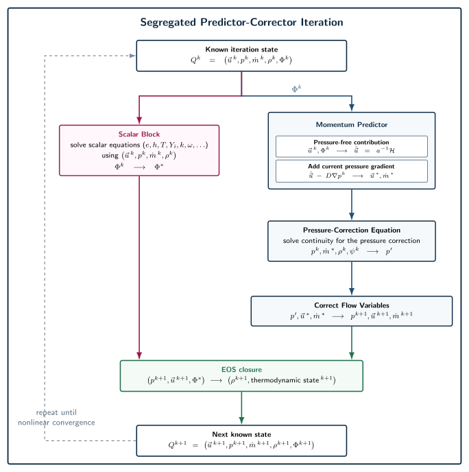
../_images/compressible_pressure_based_iteration_tikz.svg — Fig. 3.2.1 High-level information flow for one pressure-based segregated predictor-corrector iteration in the compressible solve. The arrows show the mathematical data dependence, not a strict implementation schedule for every algorithm variant.#

The figure is also the safest way to read the starred quantities in this chapter:

Symbol	How to read it in the algorithm picture
\(Q^k\)	The known state at the start of outer nonlinear iteration \(k\).
\(\Phi\)	The bundled scalar / thermochemical state, e.g. \(e\), \(h\), \(T\), \(Y_i\), and other transported scalars.
\(\Phi^*\)	The updated scalar state produced by the scalar equations during this nonlinear iteration.
\(\vec{u}^\), \(\dot{m}^\)	The momentum-predictor velocity and face flux before pressure correction.
\(p'\)	The pressure correction obtained from the pressure-correction equation built from continuity, provisional fluxes, and the EOS pressure response.
\(p^{k+1}\), \(\vec{u}^{\,k+1}\), \(\dot{m}^{\,k+1}\)	The pressure-corrected flow variables passed to the next outer iteration.
\(\rho^{k+1}\)	The density rebuilt by the EOS from the corrected pressure and updated thermodynamic state. Corrected velocity also enters when total energy or total enthalpy must be converted to a static quantity.

In pseudocode form, the same idea is:

given the converged state at time level n

for each new time level n+1:
  initialize Q^0

  for each outer nonlinear iteration k:
    solve scalar equations for Phi using the current flow state:
      (u^k, p^k, mdot^k, rho^k) -> Phi*

    assemble and solve the momentum predictor using p^k and lagged closure data:
      (u^k, p^k, rho^k, Phi^k) -> u*

    construct the pressure-coupled provisional face flux:
      (u*, p^k, momentum response) -> mhat*

    solve the pressure-correction equation from continuity, provisional fluxes, and the current EOS pressure response:
      (mhat*, rho^k, sound speed^k) -> p'

    correct pressure, velocity, and face flux
      p' -> p^{k+1}, u^{k+1}, mdot^{k+1}

    rebuild the complete EOS state using corrected pressure and Phi*
      (p^{k+1}, Phi*, and u^{k+1} when required) -> rho^{k+1}

  when the nonlinear iteration converges:
    final Q^k becomes the state at time level n+1

This picture is more important than the superscript convention. A star means “the intermediate quantity produced by the step that owns it.” Thus \(\vec{u}^*\) is a momentum-predictor velocity, while \(\Phi^*\) is a scalar-equation result. They are both intermediate quantities, but they do not mean the same stage of the algorithm.

The detailed derivations in Chapter 4, Chapter 5, and Chapter 6 show how each arrow is realized mathematically.

3.3. Notation Used In This Chapter#

The symbols below are used throughout the pressure-based algorithm discussion.

Symbol	Meaning
\(n\)	Time level. A converged time step advances the solution from \(n\) to \(n+1\).
\(k\)	Nonlinear outer-iteration level inside the new time step.
\(m\)	Pressure-corrector stage inside an outer iteration or time step.
\(\ell\)	Iteration performed by an individual linear-system solver.
\((\cdot)^*\)	Intermediate result produced by the equation block being discussed.
\((\cdot)'\)	Correction obtained from the pressure-correction equation.
\(\hat{\cdot}\)	Pressure-free contribution formed from the non-pressure part of the momentum equation.
\(P\), \(N\), \(f\)	Location labels: cell \(P\), neighboring cell \(N\), and face \(f\).
\(\left.\cdot\right\rvert_{(\cdots)}\)	Evaluation at the listed state.

A useful mental picture for one time step is

(3.3.1)#\[(\cdot)^n \;\longrightarrow\; (\cdot)^k \;\longrightarrow\; (\cdot)^* \;\longrightarrow\; (\cdot)^{k+1} \;\longrightarrow\; (\cdot)^{n+1}.\]

The star is local to the step that produces it. Thus \(\vec{u}^*\) is a momentum-predictor velocity, while \(\Phi^*\) is a scalar-equation result. They are both intermediate quantities, but they do not denote the same stage of the algorithm.

3.4. What Each Stage Contributes#

The segregated method is a block fixed-point iteration. Each equation block is linearized with coefficients and cross-equation data taken from the current outer iterate, solved for its own unknowns, and then reconciled with the other blocks through pressure correction and EOS closure. Because nonlinear coefficients and cross-couplings are lagged, this outer process is accurately described as Picard-style even when the pressure–velocity coupling inside it uses SIMPLE, SIMPLEC, or SIMPLER.

Stage	Known on entry	Principal result	What remains to be resolved
Property and scalar assembly	Current pressure, velocity, density, and closure state	Updated energy, species, turbulence, and other scalar fields	Momentum and continuity have not yet been reconciled with those changes
Momentum predictor	Current pressure and linearized momentum coefficients	Provisional cell velocity \(\vec{u}^*\)	The corresponding face flux generally violates discrete continuity
Momentum-weighted face-flux construction	Provisional velocity, pressure, and momentum response	Pressure-coupled provisional face flux \(\hat m_f^*\) and face response \(d_f\)	The pressure change required to remove the continuity defect is still unknown
Pressure-correction solve	Provisional continuity defect, \(d_f\), current density, and acoustic response	Pressure correction \(p'\)	Pressure, velocity, and face flux still have to be corrected
Primary-field correction	\(p'\) and the approximate momentum response	Corrected pressure, velocity, and face flux	The complete thermodynamic density is not yet known
EOS reconstruction	Corrected pressure, updated thermal variable and composition, and corrected velocity when total energy or enthalpy is used	Complete next-iteration thermodynamic state and \(\rho^{k+1}\)	Another outer iteration may be required for nonlinear convergence
Convergence and advance	Residuals and correction norms	Either another outer iteration or the converged state at \(n+1\)	Linear convergence alone does not imply nonlinear or time-step convergence

This table is an information-dependency map. In a rule-based implementation, independent pieces may be scheduled in a different textual order or evaluated concurrently; the mathematical contract is that every stage consumes the correct state and supplies the facts required downstream.

Solver-Anatomy Quick Reference

The momentum predictor supplies a velocity but not continuity. Momentum-weighted interpolation supplies a pressure-sensitive face flux. The pressure-correction equation chooses the pressure response needed to satisfy linearized continuity. The EOS then rebuilds the complete density from the corrected thermodynamic state. Outer iterations repeat this cycle until all coupled equations are consistent at the new physical time level.

3.5. Nested Iterations and Convergence#

Four iteration indices can appear in a practical calculation:

Index	Role
\(n\)	Physical time level, advanced only after the time-step solution is accepted
\(k\)	Outer block nonlinear iteration at the new time level
\(m\)	Pressure-corrector stage within an outer iteration or time step
\(\ell\)	Iteration of an individual linear-system solver

These indices must not be conflated. Reducing a linear residual at level \(\ell\) solves only the currently frozen algebraic row. A pressure corrector at level \(m\) reduces the discrete continuity defect for that predictor state. An outer iteration at level \(k\) reconciles the nonlinear coefficients and the different equation blocks. Only convergence of that outer process permits the solution to advance from \(n\) to \(n+1\).

3.6. Where the Detailed Machinery Is Developed#

The remainder of the opening sequence follows the data dependencies just described:

Chapter 4 derives the generic finite-volume transport row.
Chapter 5 derives the pressure-sensitive face flux used on a collocated mesh.
Chapter 6 derives the pressure-correction equation from discrete continuity.
Chapter 7 compares SIMPLE, SIMPLEC, SIMPLER, PISO, and PIMPLE after their common machinery is available.
Chapter 8 develops the nested PIMPLE predictor and corrector stages in detail.

The named algorithms change how these blocks approximate and repeat the pressure–velocity correction; they do not change the governing conservation laws developed in Chapter 2.