16. Detailed Governing Equation Forms

This appendix collects fuller forms of the core governing equations so that individual terms can be identified without jumping immediately into the finite-volume assembly. The first goal is to state the continuum carrier-phase equations with explicit source terms. The second is to show how some of those terms change appearance when the equations are rewritten for the pressure-based solver.

The source terms are kept generic on purpose. They can represent Lagrangian-particle coupling, porous-media forcing, radiation, phase change, user-specified volumetric forcing, or other model contributions. Setting them to zero gives the uncoupled carrier-flow equations. Keeping them visible is especially helpful for particle calculations, where the particle phase can deposit mass and species, exert drag on the Eulerian field, and exchange heat or phase-change energy with the carrier gas.

The intent is that, if one encounters a term such as species enthalpy diffusion, buoyancy work, a particle energy source, or a \(Dp/Dt\) coupling term while reading the theory guide or the solver implementation, there is a single place to look up what that term means and why it appears.

16.1. Common Definitions

Unless stated otherwise, the equations in the first part of this appendix are written for an inertial frame on a fixed grid. Solver-specific moving-grid and pressure-based forms are discussed later.

The principal thermodynamic quantities are

(16.1.1)\[H = h + \frac{1}{2}\vec{u}\cdot\vec{u} \qquad E = e + \frac{1}{2}\vec{u}\cdot\vec{u} \qquad h = e + \frac{p}{\rho}\]

The material derivative following the Eulerian carrier velocity is

(16.1.2)\[\frac{D}{Dt} = \frac{\partial}{\partial t} + \vec{u}\cdot\nabla\]

For a Newtonian fluid, the viscous stress tensor is

(16.1.3)\[\Matrix{\tau} = \mu \left[ \nabla \vec{u} + (\nabla \vec{u})^T - \frac{2}{3}(\nabla\cdot\vec{u})\Matrix{I} \right]\]

When turbulent transport is modeled through an eddy-viscosity assumption, the same structure is often retained with an effective viscosity \(\mu_{\mathrm{eff}}=\mu+\mu_t\).

For the additive mixture model, the species enthalpies are evaluated at the common temperature and pressure:

(16.1.4)\[h=\sum_{k=1}^{N_s}Y_kh_k(T,p)\]

Here \(h_k\) is specific enthalpy in J/kg of species \(k\); it can include real-fluid pressure dependence. The mixture assumptions and their temperature-equation consequences are developed in Temperature Equation.

For multispecies flows, the species diffusion flux is written as

(16.1.5)\[\vec{J}_k = \rho Y_k \vec{V}_k\]

Here \(\vec{V}_k\) is the diffusion velocity of species \(k\). The total heat flux is then

(16.1.6)\[\vec{q} = -\lambda \nabla T + \sum_{k=1}^{N_s} h_k \vec{J}_k\]

The first term is Fourier heat conduction. The second term is the species enthalpy diffusion term: it accounts for the fact that diffusing species carry their own enthalpy with them, so species diffusion also transports energy. Throughout this appendix, \(\vec{q}\) means the total heat flux in Eq. (16.1.6), not Fourier conduction alone.

It is also useful to define the viscous-dissipation function

(16.1.7)\[\Phi = \Matrix{\tau}:\nabla\vec{u}\]

16.2. Generic Source-Term Notation

The equations below include generic conservative source terms. These sources are written as volumetric continuum rates and are positive when they add mass, momentum, or energy to the Eulerian carrier phase. In the finite-volume implementation they may be stored temporarily as cell-integrated rates; dividing by the control-volume size recovers the continuum rate used here.

The notation used here is:

• \(S_{\rho}\): carrier-phase mass source. In a particle calculation, positive \(S_{\rho}\) means mass has moved from the Lagrangian phase into the Eulerian carrier.

• \(S_{\rho Y_k}\): species mass source for species \(k\), with \(S_{\rho}=\sum_k S_{\rho Y_k}\) when the transported species set accounts for all mass added to the carrier.

• \(\vec{S}_{\rho\vec{u}}\): conservative momentum source, with units of force per volume. Particle drag, momentum carried by transferred mass, porous-media resistance, and imposed forcing all enter this bucket.

• \(S_{\rho E}\) and \(S_{\rho H}\): conservative total-energy and total-enthalpy sources, with units of power per volume. These may include convective particle/fluid heat exchange, phase-change energy, radiation, chemistry heat release, mechanical work, or energy carried by transferred mass. For the conservative total-enthalpy equation written below, the conserved quantity is \(\rho H-p=\rho E\), so \(S_{\rho H}\) and \(S_{\rho E}\) represent the same physical source bookkeeping. Separate symbols are retained only to make contact with solver forms that use different primary variables.

• \(S_{\rho e}\) and \(S_{\rho h}\): static internal-energy and static-enthalpy sources. These are useful after a total-energy or total-enthalpy equation has been reduced to a thermal equation; they are not necessarily independent source models.

These symbols are deliberately generic. A Lagrangian particle module is one contributor, but other models can contribute to the same source buckets. A nonzero \(S_{\rho}\) is therefore not a statement that mass is created globally; in a coupled calculation it is usually an exchange between the Eulerian carrier and another modeled subsystem.

One bookkeeping point is important throughout this appendix. A conservative source \(S_{\rho\phi}\) is the source for the conserved variable \(\rho\phi\). If the same equation is rewritten for the specific variable \(\phi\), continuity contributes a correction and the source appears as \(S_{\rho\phi}-\phi S_{\rho}\). This correction is not a new physical model. It is the algebraic consequence of solving for a specific variable while the carrier continuity equation contains a mass source.

16.3. Continuity Equation

The fully compressible continuity equation is

(16.3.1)\[\frac{\partial \rho}{\partial t} + \nabla\cdot(\rho\vec{u}) = S_{\rho}\]

This equation enforces conservation of carrier-phase mass. For a closed single-phase carrier calculation, \(S_{\rho}=0\). For a coupled particle calculation, \(S_{\rho}>0\) in a cell means mass has been transferred from the Lagrangian phase into the Eulerian carrier during that instant, while \(S_{\rho}<0\) would represent removal from the carrier.

For compressible flows, density is not independent; it is obtained from an equation of state,

(16.3.2)\[\rho = \rho(p,T,Y_k,\ldots)\]

For ideal-gas mixtures this reduces to \(\rho = p/(R_m T)\), while for real-fluid calculations the same continuity equation remains valid but the thermodynamic closure is more general.

16.4. Momentum Equation

A convenient full form of the momentum equation is

(16.4.1)\[\frac{\partial (\rho \vec{u})}{\partial t} + \nabla\cdot(\rho\vec{u}\otimes\vec{u}) = -\nabla p + \nabla\cdot\Matrix{\tau} + \vec{f}_b + \vec{f}_{ni} + \vec{S}_{\rho\vec{u}}\]

The terms on the right-hand side are:

• \(-\nabla p\): pressure-gradient force.

• \(\nabla\cdot\Matrix{\tau}\): viscous diffusion of momentum.

• \(\vec{f}_b\): body-force contribution associated with gravity or buoyancy.

• \(\vec{f}_{ni}\): non-inertial reference-frame forces such as Coriolis, centrifugal, angular-acceleration, or translational-acceleration terms.

• \(\vec{S}_{\rho\vec{u}}\): any additional model-dependent conservative momentum source, including particle drag, momentum carried by mass transfer, porous-media resistance, or user-specified forcing.

A dedicated derivation of the non-inertial kinematics and apparent-force terms is given in the non-inertial reference-frame appendix.

For buoyant flows, the same physics is sometimes written as \(\rho\vec{g}\) and sometimes as \((\rho-\rho_{\mathrm{ref}})\vec{g}\), depending on how the hydrostatic part of the pressure field is handled. The governing physics is the same; only the pressure-force decomposition changes.

For particle coupling, \(\vec{S}_{\rho\vec{u}}\) is the momentum received by the carrier per unit volume and time. With the sign convention above, a drag force exerted by the particles on the gas enters with the sign of the force on the gas.

16.5. Total Enthalpy Equation

The total enthalpy form is often the most direct way to see where pressure work has gone. A useful continuum form is

(16.5.1)\[\frac{\partial(\rho H - p)}{\partial t} + \nabla\cdot(\rho\vec{u}H) = -\nabla\cdot\vec{q} + \nabla\cdot(\Matrix{\tau}\cdot\vec{u}) + \vec{f}_b\cdot\vec{u} + \vec{f}_{ni}\cdot\vec{u} + S_{\rho H}\]

Here \(\vec{q}\) is the total heat flux defined in Eq. (16.1.6). In multispecies calculations, this means that the compact term \(-\nabla\cdot\vec{q}\) already includes the species enthalpy diffusion contribution associated with the species fluxes \(\vec{J}_k\) from Eq. (16.1.5).

Substituting the total heat-flux definition gives

(16.5.2)\[\frac{\partial(\rho H - p)}{\partial t} + \nabla\cdot(\rho\vec{u}H) = \nabla\cdot(\lambda\nabla T) - \nabla\cdot\left(\sum_{k=1}^{N_s} h_k \vec{J}_k\right) + \nabla\cdot(\Matrix{\tau}\cdot\vec{u}) + \vec{f}_b\cdot\vec{u} + \vec{f}_{ni}\cdot\vec{u} + S_{\rho H}\]

The important physical terms are:

• \(\nabla\cdot(\lambda\nabla T)\): thermal conduction.

• \(-\nabla\cdot\left(\sum h_k \vec{J}_k\right)\): species enthalpy diffusion.

• \(\nabla\cdot(\Matrix{\tau}\cdot\vec{u})\): viscous work.

• \(\vec{f}_b\cdot\vec{u}\) and \(\vec{f}_{ni}\cdot\vec{u}\): work done by body forces.

• \(S_{\rho H}\): any additional conservative total-enthalpy source such as chemistry, radiation, phase change, particle/fluid heat exchange, or user-specified source models.

If a model transfers mass into the carrier, the enthalpy source should be interpreted as the conservative enthalpy rate delivered to the carrier before any later specific-variable correction is applied. For example, an evaporating particle may contribute both species mass and the enthalpy associated with the vapor it deposits.

Because the conserved variable in this form is \(\rho H-p=\rho E\), this conservative source is the same physical source that appears in the total-energy equation, i.e. \(S_{\rho H}\equiv S_{\rho E}\) for the continuum equation as written here. Differences between total-enthalpy and total-energy solver rows arise later from rewriting the equation for a specific primary variable and from moving pressure terms between the left- and right-hand sides.

16.6. Total Energy Equation

The total energy equation can be written as

(16.6.1)\[\frac{\partial(\rho E)}{\partial t} + \nabla\cdot(\rho\vec{u}H) = -\nabla\cdot\vec{q} + \nabla\cdot(\Matrix{\tau}\cdot\vec{u}) + \vec{f}_b\cdot\vec{u} + \vec{f}_{ni}\cdot\vec{u} + S_{\rho E}\]

As in the total enthalpy form, \(\vec{q}\) is the total heat flux in Eq. (16.1.6). The expanded form therefore contains both Fourier heat conduction and species enthalpy diffusion:

(16.6.2)\[\frac{\partial(\rho E)}{\partial t} + \nabla\cdot(\rho\vec{u}H) = \nabla\cdot(\lambda\nabla T) - \nabla\cdot\left(\sum_{k=1}^{N_s} h_k \vec{J}_k\right) + \nabla\cdot(\Matrix{\tau}\cdot\vec{u}) + \vec{f}_b\cdot\vec{u} + \vec{f}_{ni}\cdot\vec{u} + S_{\rho E}\]

An equivalent split form that makes the pressure-work term explicit is

(16.6.3)\[\frac{\partial(\rho E)}{\partial t} + \nabla\cdot(\rho\vec{u}E) = -\nabla\cdot(p\vec{u}) - \nabla\cdot\vec{q} + \nabla\cdot(\Matrix{\tau}\cdot\vec{u}) + \vec{f}_b\cdot\vec{u} + \vec{f}_{ni}\cdot\vec{u} + S_{\rho E}\]

This equation and the total enthalpy equation are algebraically equivalent; the difference is only how the pressure-related transport is grouped. The heat-flux meaning is unchanged: \(-\nabla\cdot\vec{q}\) still includes the species enthalpy diffusion term from Eq. (16.1.6).

For particle coupling, \(S_{\rho E}\) is the conservative total-energy rate delivered to the carrier. It may contain thermal exchange, phase-change energy, energy carried by transferred mass, and mechanical work associated with interphase momentum exchange. Which part of that total source later appears as heat in the temperature equation depends on the kinetic-energy bookkeeping described next.

16.7. Temperature Equation

The temperature equation follows from conservation of energy and the thermodynamic relation between enthalpy, temperature, pressure, and composition[Pan96]. We consider an ideal mixture whose species share a common temperature and pressure, with additive enthalpy:

(16.7.1)\[h(T,p,Y)=\sum_{k=1}^{N_s}Y_k h_k(T,p) \qquad \sum_{k=1}^{N_s}Y_k=1\]

Each species enthalpy \(h_k\) depends on \(T\) and \(p\), but not on composition. The species may have real-fluid properties; no ideal-gas pressure-density relation or constant specific heat is assumed. All thermodynamic properties and source energies use consistent energy references. All \(N_s\) species balances are retained, as is the continuity source \(S_\rho\).

16.7.1. From Total Energy To Static Enthalpy

Let \(K=\tfrac12\vec u\cdot\vec u\) and \(E=e+K\). Dotting the momentum balance with \(\vec u\) and using continuity gives the kinetic-energy source

(16.7.1.1)\[S_K=\vec u\cdot\vec S_{\rho\vec u}-KS_\rho\]

Subtracting the kinetic-energy balance from total energy leaves

(16.7.1.2)\[\begin{split}\begin{aligned} \frac{\partial(\rho e)}{\partial t} +\nabla\cdot(\rho\vec u e) &=-p\nabla\cdot\vec u-\nabla\cdot\vec q+\Phi+S_{\rho e}\\ S_{\rho e}&=S_{\rho E}-\vec u\cdot\vec S_{\rho\vec u}+KS_\rho \end{aligned}\end{split}\]

Here \(\vec q\) includes conduction and species enthalpy diffusion, as in Eq. (16.1.6), and \(\Phi=\Matrix{\tau}:\nabla\vec u\) is viscous dissipation. The source \(S_{\rho e}\) is the energy transfer remaining after the work that changes carrier kinetic energy has been removed.

Since \(\rho h=\rho e+p\), adding the transport of \(p\) gives the static enthalpy balance. Its material form follows from \(\partial_t(\rho h)+\nabla\cdot(\rho\vec u h)=\rho Dh/Dt+hS_\rho\):

(16.7.1.3)\[\begin{split}\begin{aligned} \frac{\partial(\rho h)}{\partial t}+\nabla\cdot(\rho\vec u h) &=\frac{Dp}{Dt}-\nabla\cdot\vec q+\Phi+S_{\rho e}\\ \rho\frac{Dh}{Dt} &=\frac{Dp}{Dt}-\nabla\cdot\vec q+\Phi+S_{\rho e}-hS_\rho \end{aligned}\end{split}\]

16.7.2. From Enthalpy To Temperature

Define the mixture specific heat and isobaric expansion coefficient by

(16.7.2.1)\[c_p=\left(\frac{\partial h}{\partial T}\right)_{p,Y} \qquad \beta_T=-\frac1\rho\left(\frac{\partial\rho}{\partial T}\right)_{p,Y}\]

For a thermodynamically consistent EOS, \((\partial h/\partial p)_{T,Y}=(1-\beta_TT)/\rho\). Differentiating the additive enthalpy relation therefore gives

(16.7.2.2)\[dh=c_p\,dT+\frac{1-\beta_TT}{\rho}\,dp +\sum_{k=1}^{N_s}h_k\,dY_k\]

The three contributions represent changes in temperature, pressure, and composition. Substitution into Eq. (16.7.1.3) gives

(16.7.2.3)\[\rho c_p\frac{DT}{Dt}-\beta_TT\frac{Dp}{Dt} =-\nabla\cdot\vec q+\Phi+S_{\rho e}-hS_\rho -\rho\sum_{k=1}^{N_s}h_k\frac{DY_k}{Dt}\]

The last term accounts for the part of an enthalpy change caused by changing composition rather than temperature.

16.7.3. Species Balances And The Temperature Source

For each species, its conservative balance and continuity give

(16.7.3.1)\[\begin{split}\begin{aligned} \frac{\partial(\rho Y_k)}{\partial t}+\nabla\cdot(\rho\vec uY_k) &=-\nabla\cdot\vec J_k+\dot\omega_k+S_{\rho Y_k}\\ \rho\frac{DY_k}{Dt} &=-\nabla\cdot\vec J_k+\dot\omega_k+S_{\rho Y_k}-Y_kS_\rho \end{aligned}\end{split}\]

Here \(\vec J_k\) is the diffusion mass flux relative to the mixture velocity, in kg/(m\(^2\) s); \(\dot\omega_k\) is chemical production, and \(S_{\rho Y_k}\) is external species mass addition, both in kg/(m\(^3\) s). Mixture conservation requires

(16.7.3.2)\[\sum_kY_k=1\qquad \sum_k\vec J_k=\vec0\qquad \sum_k\dot\omega_k=0\qquad \sum_kS_{\rho Y_k}=S_\rho\]

All sums run over the \(N_s\) species. Their balances sum to continuity. Multiplying the material species balances by \(-h_k\) and summing gives

(16.7.3.3)\[-\rho\sum_k h_k\frac{DY_k}{Dt} =\sum_k h_k\nabla\cdot\vec J_k -\sum_k h_k(\dot\omega_k+S_{\rho Y_k})+hS_\rho\]

The \(+hS_\rho\) cancels the \(-hS_\rho\) in Eq. (16.7.2.3). Substituting \(\vec q=-\lambda\nabla T+\sum_kh_k\vec J_k\) then combines the species-diffusion terms:

(16.7.3.4)\[-\nabla\cdot\left(\sum_kh_k\vec J_k\right) +\sum_kh_k\nabla\cdot\vec J_k =-\sum_k\vec J_k\cdot\nabla h_k\]

The sources remaining after this conversion define \(S_T\), in W/m\(^3\):

(16.7.3.5)\[\begin{split}\begin{aligned} S_T&=S_{\rho e}-\sum_kh_k(\dot\omega_k+S_{\rho Y_k})\\ &=S_{\rho E}-\vec u\cdot\vec S_{\rho\vec u}+KS_\rho -\sum_kh_k(\dot\omega_k+S_{\rho Y_k}) \end{aligned}\end{split}\]

Mass addition remains through these energy, momentum, and species sources. When species enthalpies include formation energies, \(-\sum_kh_k\dot\omega_k\) supplies the temperature-form reaction source; adding the same reaction heat to \(S_{\rho E}\) would count it twice.

Temperature Equation

(16.7.3.6)\[\rho c_p\frac{DT}{Dt} =\beta_TT\frac{Dp}{Dt}+\nabla\cdot(\lambda\nabla T) -\sum_k\vec J_k\cdot\nabla h_k+\Phi+S_T\]

Every term has units of power per volume. Their meanings are:

Term	Contribution
\(\rho c_pDT/Dt\)	Enthalpy change due to temperature change following the mixture.
\(\beta_TT\,Dp/Dt\)	Pressure work after converting enthalpy to temperature.
\(\nabla\cdot(\lambda\nabla T)\)	Fourier conduction, with thermal conductivity \(\lambda\).
\(-\sum_k\vec J_k\cdot\nabla h_k\)	Species enthalpy transport combined with its composition conversion.
\(\Phi\)	Viscous dissipation.
\(S_T\)	Energy and species source conversion defined above.

16.7.4. Species Enthalpy Diffusion

The two terms on the left of Eq. (16.7.3.4) have different roles. The first is species enthalpy transport: energy carried by the diffusing species. The second is composition conversion: subtraction of the enthalpy change already represented by the changing species masses. A total-enthalpy balance receives the energy flux directly; temperature requires both contributions.

The zero-sum mass-flux condition does not cancel enthalpy transport. For two species with \(\vec J_1=\vec J\) and \(\vec J_2=-\vec J\), the enthalpy flux is \((h_1-h_2)\vec J\). At uniform temperature and pressure, each \(\nabla h_k=0\), so the two contributions cancel in the temperature balance even though energy can move between cells.

For comparison with a species-specific-heat expression, define \(c_{p,k}=(\partial h_k/\partial T)_p\). Additive mixing gives \(c_p=\sum_kY_kc_{p,k}\), but the species enthalpy gradient also contains its pressure dependence:

(16.7.4.1)\[\nabla h_k=c_{p,k}\nabla T +\left(\frac{\partial h_k}{\partial p}\right)_T\nabla p\]

Consequently,

(16.7.4.2)\[-\sum_k\vec J_k\cdot\nabla h_k =-\sum_kc_{p,k}\vec J_k\cdot\nabla T -\sum_k\left(\frac{\partial h_k}{\partial p}\right)_T \vec J_k\cdot\nabla p\]

Retaining \(\nabla h_k\) includes both contributions without separately evaluating species heat capacities or pressure derivatives. The pressure contribution is distinct from the mixture pressure-work term \(\beta_TT\,Dp/Dt\); neither replaces the other.

When species enthalpies are pressure independent, as in an ideal-gas mixture, or when pressure is spatially uniform, the species contribution reduces to

(16.7.4.3)\[-\sum_kc_{p,k}\vec J_k\cdot\nabla T\]

This species-specific-heat form contains both species enthalpy transport and composition conversion.

With a Fick flux \(\vec J_k=-\rho D_k\nabla Y_k\) that satisfies \(\sum_k\vec J_k=\vec0\), this is

(16.7.4.4)\[\rho\sum_kD_kc_{p,k}\nabla Y_k\cdot\nabla T\]

Here \(D_k\) is species mass diffusivity. If a mass-conservation correction is applied to the Fick flux, that corrected flux must also be used in Eq. (16.7.4.3). The ideal-gas specialization additionally has \(\beta_TT=1\) in the pressure-work term.

If a heat-flux model omits species enthalpy transport while retaining species diffusion, only the first term on the left of Eq. (16.7.3.4) is omitted. The composition contribution remains, and isothermal cancellation no longer generally holds.

16.7.5. Division By The Mixture Specific Heat

With the species enthalpy flux \(\vec q_h^{\mathrm{diff}}=\sum_kh_k\vec J_k\), the temperature balance is

(16.7.5.1)\[\begin{split}\begin{aligned} \rho c_p\frac{DT}{Dt}=Q_T &=-\nabla\cdot\vec q_h^{\mathrm{diff}} +\sum_kh_k\nabla\cdot\vec J_k\\ &\quad+\nabla\cdot(\lambda\nabla T) +\beta_TT\frac{Dp}{Dt}+\Phi+S_T \end{aligned}\end{split}\]

Here \(Q_T\) denotes the complete right-hand side, in W/m\(^3\). Dividing every term by the mixture specific heat gives

(16.7.5.2)\[\begin{split}\begin{aligned} \rho\frac{DT}{Dt}=\frac{Q_T}{c_p} &=-\frac1{c_p}\nabla\cdot\vec q_h^{\mathrm{diff}} +\frac1{c_p}\sum_kh_k\nabla\cdot\vec J_k\\ &\quad+\frac1{c_p}\nabla\cdot(\lambda\nabla T) +\frac{\beta_TT}{c_p}\frac{Dp}{Dt}+\frac{\Phi+S_T}{c_p} \end{aligned}\end{split}\]

Each term now has units of kg K/(m\(^3\) s). The factor \(1/c_p\) multiplies each complete flux divergence. It can also be included in the flux by using the product rule. For a contribution \(+\nabla\cdot\vec F\), where \(\vec F\) is an energy flux in W/m\(^2\),

(16.7.5.3)\[\frac1{c_p}\nabla\cdot\vec F =\nabla\cdot\left(\frac{\vec F}{c_p}\right) + \frac{\vec F\cdot\nabla c_p}{c_p^2}\]

For species enthalpy transport, \(\vec F=-\vec q_h^{\mathrm{diff}}\), so

(16.7.5.4)\[-\frac1{c_p}\nabla\cdot\vec q_h^{\mathrm{diff}} =-\nabla\cdot\left(\frac{\vec q_h^{\mathrm{diff}}}{c_p}\right) -\frac{\vec q_h^{\mathrm{diff}}\cdot\nabla c_p}{c_p^2}\]

The left-hand form evaluates the enthalpy-flux divergence and then divides by local \(c_p\). The right-hand form uses the flux \(\vec q_h^{\mathrm{diff}}/c_p\) and the gradient of \(c_p\). Including the composition contribution gives

(16.7.5.5)\[\frac1{c_p}\left[-\nabla\cdot\vec q_h^{\mathrm{diff}} +\sum_kh_k\nabla\cdot\vec J_k\right] =-\frac1{c_p}\sum_k\vec J_k\cdot\nabla h_k\]

For conduction, \(\vec F=\lambda\nabla T\). Applying the same product rule and combining the species contributions gives

(16.7.5.6)\[\begin{aligned} \rho\frac{DT}{Dt} &=\nabla\cdot\left(\frac{\lambda}{c_p}\nabla T\right) +\frac{\lambda}{c_p^2}\nabla c_p\cdot\nabla T -\frac1{c_p}\sum_k\vec J_k\cdot\nabla h_k + \frac{\beta_TT}{c_p}\frac{Dp}{Dt}+\frac{\Phi+S_T}{c_p} \end{aligned}\]

Constant mixture \(c_p\) removes the product-rule corrections; it does not remove composition conversion. Even constant species heat capacities can give a varying mixture \(c_p\) when composition varies.

The conservative transport of \(\rho T\) also contains the continuity source:

(16.7.5.7)\[\frac{\partial(\rho T)}{\partial t}+\nabla\cdot(\rho\vec uT) =\frac{Q_T}{c_p}+TS_\rho\]

Subtracting \(T\) times continuity recovers \(\rho DT/Dt=Q_T/c_p\). The alternative transport of \(\rho c_pT\) is developed in the solver-form discussion.

16.7.6. Turbulent Temperature Transport

An overbar denotes Reynolds averaging, and a tilde denotes Favre averaging: \(\widetilde\phi=\overline{\rho\phi}/\bar\rho\) and \(\phi=\widetilde\phi+\phi''\). Averaging the conservative equation gives

(16.7.6.1)\[\frac{\partial(\bar\rho\widetilde T)}{\partial t} +\nabla\cdot(\bar\rho\widetilde{\vec u}\widetilde T) =-\nabla\cdot\overline{\rho\vec u''T''} +\overline{\frac{Q_T}{c_p}}+\overline{TS_\rho}\]

The averaging steps are given in Averaging the Temperature Equation. The turbulent temperature flux is modeled by

(16.7.6.2)\[-\overline{\rho\vec u''T''}\approx\frac{\mu_t}{Pr_t}\nabla\widetilde T\]

Here \(\mu_t\) is turbulent dynamic viscosity and \(Pr_t\) the turbulent Prandtl number. A mean-state closure also evaluates properties at \((\widetilde T,\bar p,\widetilde Y)\) and represents the averaged species contribution using the modeled species flux \(\vec J_k^{\,\mathrm{mod}}\). This flux includes molecular and turbulent diffusion, with the same mass-conservation correction used in the mean species balances.

With these approximations, the temperature equation takes the form

(16.7.6.3)\[\begin{split}\begin{aligned} \bar\rho\frac{D\widetilde T}{Dt} &\approx\nabla\cdot\left[\left(\frac{\lambda}{c_p} +\frac{\mu_t}{Pr_t}\right)\nabla\widetilde T\right] +\frac{\lambda}{c_p^2}\nabla c_p\cdot\nabla\widetilde T\\ &\quad-\frac1{c_p}\sum_k\vec J_k^{\,\mathrm{mod}}\cdot\nabla h_k +\frac{\beta_T\widetilde T}{c_p}\frac{D\bar p}{Dt} +\frac{\Phi+S_T}{c_p}+\overline{T''S_\rho} \end{aligned}\end{split}\]

Here \(D/Dt=\partial_t+\widetilde{\vec u}\cdot\nabla\). Unmarked properties, \(\Phi\), and \(S_T\) are evaluated or modeled at the mean state; this replaces correlations in \(\overline{Q_T/c_p}\) and is a modeling approximation. The remaining mass-source correlation must be modeled or explicitly neglected. Setting it to zero amounts to assuming \(\overline{TS_\rho}\approx\widetilde T\,\overline{S_\rho}\).

Only molecular conductivity appears in the \(\nabla c_p\) correction, because the turbulent closure acts directly on temperature flux:

(16.7.6.4)\[\begin{split}\begin{aligned} \frac1{c_p}\nabla\cdot(\lambda\nabla\widetilde T) +\nabla\cdot\left(\frac{\mu_t}{Pr_t}\nabla\widetilde T\right) &=\nabla\cdot\left[\left(\frac{\lambda}{c_p} +\frac{\mu_t}{Pr_t}\right)\nabla\widetilde T\right]\\ &\quad+\frac{\lambda}{c_p^2}\nabla c_p\cdot\nabla\widetilde T \end{aligned}\end{split}\]

Dividing the divergence of a modeled turbulent enthalpy flux by \(c_p\) would instead introduce a turbulent \(\nabla c_p\) contribution. That is a different closure when \(c_p\) varies.

16.7.7. Finite-Volume Species Diffusion

For an interior face shared by cells \(L\) and \(R\), the stored area vector \(\vec S_f\) points from \(L\) to \(R\). Define the signed species mass flow rate \(F_{k,f}=\vec J_{k,f}\cdot\vec S_f\), in kg/s. The incidence sign \(\sigma_{Pf}\) is \(+1\) for \(P=L\) and \(-1\) for \(P=R\); an outward boundary face uses \(+1\), as in Loci Face Orientation and Cell Incidence.

Conservative species reconstruction and diffusion enforce \(\sum_kY_{k,f}=1\) and \(\sum_kF_{k,f}=0\). The same corrected diffusion rates enter the energy balance. Each species carries an enthalpy rate

(16.7.7.1)\[F_{hY,k,f}=h_{k,f}F_{k,f}\]

A limited reconstruction from each adjacent cell gives

(16.7.7.2)\[h_{k,f}^{(P)}=h_{k,P} +\Psi_{h,k,P}\nabla h_{k,P}\cdot(\vec x_f-\vec x_P)\qquad P=L,R\]

Here \(\Psi_{h,k,P}\) is the limiter and \(\vec x\) denotes a centroid. A centered face value is

(16.7.7.3)\[h_{k,f}\approx\tfrac12\left(h_{k,f}^{(L)}+h_{k,f}^{(R)}\right)\]

This value is independent of the bulk advection direction: species can diffuse when that velocity is zero or changes sign. Both cells use the same face enthalpy rate with opposite signs.

The cell-integrated diffusion contributions to species mass and enthalpy are, respectively,

(16.7.7.4)\[R_{k,P}^{\mathrm{diff}}=-\sum_f\sigma_{Pf}F_{k,f}\qquad Q_{h,P}^{\mathrm{diff}}=-\sum_f\sigma_{Pf}\sum_kh_{k,f}F_{k,f}\]

The first has units of kg/s and the second of W. Total enthalpy receives \(Q_{h,P}^{\mathrm{diff}}\) directly. Temperature requires the composition conversion as well:

(16.7.7.5)\[\begin{split}\begin{aligned} Q_{T,P}^{\mathrm{diff}} &=Q_{h,P}^{\mathrm{diff}}-\sum_kh_{k,P}R_{k,P}^{\mathrm{diff}}\\ &=-\sum_f\sigma_{Pf}\sum_k(h_{k,f}-h_{k,P})F_{k,f} \end{aligned}\end{split}\]

Dividing this power by \(c_{p,P}\) gives the specific-temperature contribution, in kg K/s, corresponding to Eq. (16.7.5.5). Keeping cell \(1/c_{p,P}\) outside the enthalpy-flux sum retains the left-hand side of Eq. (16.7.5.4); face scaling would require its product-rule correction. Both numerator terms must use the same species mass flow rates.

At uniform temperature and pressure, \(h_{k,f}=h_{k,P}\) and each species contribution vanishes. If species enthalpy transport is omitted from the heat-flux model, only \(Q_{h,P}^{\mathrm{diff}}\) is removed; the composition contribution remains. Conservation over finite changes in temperature and composition also depends on time and convection discretization, as discussed in Temperature And Discrete Energy Conservation.

16.7.8. Example: Mass Deposition

Suppose mass is deposited at volumetric rate \(\dot m\) with velocity \(\vec u_m\) and composition \(Y_{k,m}\). If \(S_{\mathrm{stat},m}\) is the non-kinetic energy supplied by the deposition model, the conservative sources are

(16.7.8.1)\[S_\rho^{\,m}=\dot m\qquad \vec S_{\rho\vec u}^{\,m}=\dot m\vec u_m\qquad S_{\rho Y_k}^{\,m}=\dot mY_{k,m}\qquad S_{\rho E}^{\,m}=S_{\mathrm{stat},m}+\tfrac12\dot m|\vec u_m|^2\]

Here \(\sum_kY_{k,m}=1\). Removing the carrier kinetic-energy contribution gives \(S_{\rho e}^{\,m}=S_{\mathrm{stat},m} +\tfrac12\dot m|\vec u_m-\vec u|^2\). The temperature source is therefore

(16.7.8.2)\[S_T^{\,m}=S_{\mathrm{stat},m} +\tfrac12\dot m|\vec u_m-\vec u|^2 -\dot m\sum_kh_k(T,p)Y_{k,m}\]

The species enthalpies are evaluated at the receiving fluid’s temperature and pressure. Mass arriving at the carrier velocity has no relative kinetic-energy contribution. If its composition also matches the carrier, the last term is \(-h\dot m\). Division by \(c_p\) gives the source in the specific-temperature equation.

16.8. Species Equation

For each transported species,

(16.8.1)\[\frac{\partial(\rho Y_k)}{\partial t} + \nabla\cdot(\rho\vec{u}Y_k) = -\nabla\cdot\vec{J}_k + \dot{\omega}_k + S_{\rho Y_k} \qquad k=1,\ldots,N_s\]

The term \(-\nabla\cdot\vec{J}_k\) is species diffusion, \(\dot{\omega}_k\) is the net production or destruction rate due to chemistry or other inter-species source mechanisms, and \(S_{\rho Y_k}\) is a generic species mass source. In a particle evaporation calculation, for example, the particle model deposits mass into the gas species selected by the evaporation or boiling model. The species equations are coupled back into the energy equations through the diffusion fluxes \(\vec{J}_k\), the species enthalpies \(h_k\), and any enthalpy associated with \(S_{\rho Y_k}\).

The constraints in Eq. (16.7.3.2) ensure that the sum of these equations is continuity. Their enthalpy-weighted sum supplies the temperature conversion in Eq. (16.7.3.3).

16.9. Solver-Form Notes

The equations above are the continuum reference forms. In the solver, additional terms can appear when the equations are written in forms that are more convenient for pressure-based finite-volume discretization. Those terms are not new physics; they arise from rewriting, linearization, or discrete bookkeeping.

16.9.1. Moving-Grid Form

On moving or deforming grids, the convective transport is written in terms of the velocity relative to the grid,

(16.9.1.1)\[\vec{u}_r = \vec{u} - \vec{u}_g\]

A term like \(\nabla\cdot(\rho\vec{u}\phi)\) becomes \(\nabla\cdot(\rho\vec{u}_r\phi)\). This is the ALE form of the transport equations.

For the generic transport identities below, define the corresponding transport derivative

(16.9.1.2)\[\frac{D_r\phi}{Dt} = \frac{\partial \phi}{\partial t} + \vec{u}_r\cdot\nabla\phi\]

On a fixed grid, \(\vec{u}_r=\vec{u}\) and \(D_r/Dt\) reduces to the material derivative \(D/Dt\) used earlier.

16.9.2. Continuity-Added Transport Form

For a generic transported variable \(\phi\),

(16.9.2.1)\[\frac{\partial(\rho\phi)}{\partial t} + \nabla\cdot(\rho\vec{u}_r\phi) = \rho\frac{\partial \phi}{\partial t} + \rho\vec{u}_r\cdot\nabla\phi + \phi\left[ \frac{\partial \rho}{\partial t} + \nabla\cdot(\rho\vec{u}_r) \right]\]

If \(S_{\rho}=0\), the bracketed term vanishes at the continuum level by continuity. In a discrete solver, however, one may choose either the conservative form or the continuity-added form because the resulting linear systems have different properties. The extra terms that show up in the discrete equations are therefore associated with the chosen transport form, not with additional physical modeling.

When continuity has a source, the bracketed term is \(S_{\rho}\) rather than zero. Consider the conservative transport equation

(16.9.2.2)\[\frac{\partial(\rho\phi)}{\partial t} + \nabla\cdot(\rho\vec{u}_r\phi) = \mathcal{L}_{\phi} + S_{\rho\phi}\]

The corresponding specific-variable form is

(16.9.2.3)\[\rho\frac{D_r\phi}{Dt} = \mathcal{L}_{\phi} + S_{\rho\phi} - \phi S_{\rho}\]

This is the source-bookkeeping pattern used by the Lagrangian-particle coupling. The particle module contributes conservative mass, species, momentum, and energy transfer rates; the specific-variable rewrite then introduces \(-\phi S_{\rho}\) for quantities such as velocity, total enthalpy, total energy, or species mass fraction. Temperature additionally requires the EOS and species conversion derived in From Enthalpy To Temperature.

16.9.3. Why Pressure-Time Terms May Appear Explicitly

In the total enthalpy equation, the conserved quantity is \(\rho H-p\). When this equation is discretized, it is common to keep the transported unknown as \(H\) and move the pressure part to the right-hand side. That is why a temporal pressure-derivative contribution can appear explicitly in the assembled equation even though it originated from the basic continuum form.

Similarly, in the temperature equation the \(Dp/Dt\) term is not an artificial source term. It is part of the thermodynamic temperature equation itself. What changes in the solver is only how that term is evaluated and linearized.

16.9.4. Conservative \(\rho c_pT\) Transport

For \(Q_T\) defined in Eq. (16.7.5.1), transport of \(c_pT\) gives

(16.9.4.1)\[\begin{split}\begin{aligned} \frac{\partial(\rho c_pT)}{\partial t} +\nabla\cdot(\rho\vec u c_pT) &=\rho c_p\frac{DT}{Dt}+\rho T\frac{Dc_p}{Dt}+c_pTS_\rho\\ &=Q_T+\rho T\frac{Dc_p}{Dt}+c_pTS_\rho \end{aligned}\end{split}\]

The derivative \(Dc_p/Dt\) includes temperature, pressure, and composition changes. Subtracting continuity multiplied by \(c_pT\) removes \(c_pTS_\rho\) but leaves \(\rho T\,Dc_p/Dt\).

The external-source contribution to this conservative form is

(16.9.4.2)\[S_{tt,\mathrm{model}}=S_{\rho E}-\vec u\cdot\vec S_{\rho\vec u}+KS_\rho -\sum_kh_kS_{\rho Y_k}+c_pTS_\rho\]

It has units of W/m\(^3\). Chemistry contributes \(-\sum_kh_k\dot\omega_k\) separately. Continuity subtraction removes the last term of \(S_{tt,\mathrm{model}}\), recovering the external part of Eq. (16.7.3.5).

16.9.5. Temperature And Discrete Energy Conservation

The temperature and total-enthalpy equations describe the same continuum energy balance when their thermodynamic conversions and source terms are complete. Their numerical approximations can nevertheless conserve energy differently. A temperature change represents an energy change through the EOS; the energy change depends on the initial and final temperature, composition, and pressure.

16.9.5.1. A Differential And A Finite Change

Consider an ideal-gas mixture with constant individual species heat capacities. For this example, set every species reference enthalpy to zero at the same temperature \(T_0\), and write \(\theta=T-T_0\). Then

(16.9.5.1)\[h_k=c_{p,k}\theta\qquad c_p=\sum_{k=1}^{N_s}Y_kc_{p,k}\qquad h=c_p\theta\]

The mixture \(c_p\) can change as the species fractions change, even though each \(c_{p,k}\) is constant. The differential identity is

(16.9.5.2)\[dh=c_p\,dT+\theta\,dc_p =c_p\,dT+\sum_{k=1}^{N_s}h_k\,dY_k\]

For two finite states, define \(\Delta T=T^{n+1}-T^n\) and \(\Delta c_p=c_p^{n+1}-c_p^n\). Expanding the product gives

(16.9.5.3)\[\begin{split}\begin{aligned} \Delta h &=(c_p^n+\Delta c_p)(\theta^n+\Delta T)-c_p^n\theta^n \\ &=c_p^n\Delta T+\theta^n\Delta c_p+\Delta c_p\Delta T \end{aligned}\end{split}\]

The last product is the energy associated with changing both quantities. It follows from multiplication of the two finite changes. In a derivative, for smooth changes over \(\Delta t\), this product is of order \((\Delta t)^2\); after division by \(\Delta t\) it vanishes as \(\Delta t\rightarrow0\). Thus it does not appear as an additional term in the exact differential identity.

Using the new-state coefficients for both contributions gives

(16.9.5.4)\[c_p^{n+1}\Delta T+\theta^{n+1}\Delta c_p =\Delta h+\Delta c_p\Delta T\]

Both contributions now include the change shared by temperature and heat capacity. Adding them counts that part twice, as illustrated below.

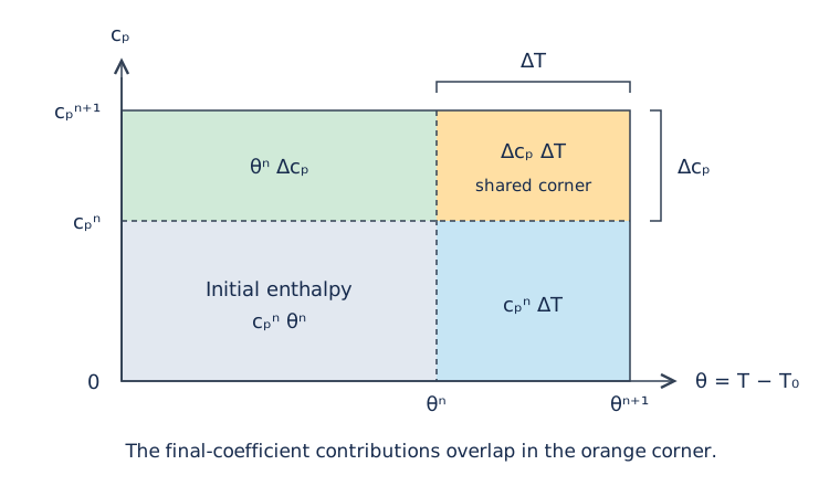
Fig. 16.9.5.1 The product \(h=c_p\theta\) represented as an area. The upper-right corner is included in both \(c_p^{n+1}\Delta T\) and \(\theta^{n+1}\Delta c_p\). Subtracting it once gives the actual change in area. The drawing shows positive changes; the algebra also holds for signed changes.

For example, let \(c_p\) increase from 1 to 2 kJ/(kg K), while \(\theta\) increases from 10 to 20 K. These values illustrate the arithmetic; they do not represent a prediction for a particular flow.

Quantity	Initial state	Final state
\(c_p\), kJ/(kg K)	1	2
\(\theta\), K	10	20
\(h=c_p\theta\), kJ/kg	10	40

The actual enthalpy increase is 30 kJ/kg. Using both final coefficients gives \(2\times10+20\times1=40\) kJ/kg. The excess 10 kJ/kg is exactly \(\Delta c_p\Delta T\).

Finite differences can also satisfy an exact product identity. For the same example,

(16.9.5.5)\[\Delta h=c_p^{n+1}\Delta T+\theta^n\Delta c_p\]

This expression first changes composition at the initial temperature, then changes temperature using the final composition. It accounts for each part once. It illustrates consistent finite-change accounting; it is not a general time-integration prescription for an arbitrary EOS.

Allowing constant, nonzero species reference enthalpies leaves the endpoint identity in the form

(16.9.5.6)\[c_p^{n+1}\Delta T +\sum_{k=1}^{N_s}h_k^{n+1}\Delta Y_k =\Delta h+\Delta c_p\Delta T\]

Here all \(N_s\) species are retained, with \(\sum_k\Delta Y_k=0\). For a general caloric EOS, the finite enthalpy change need not have this bilinear form. The appropriate reference is the difference of EOS enthalpies at the two states.

16.9.5.2. Why The Conserved Energy Balance Is Different

Total enthalpy transport also contains products, including \(\rho H\) and \(\dot m_fH_f\). Its conservation property follows from the assembled balance of complete stored energies and shared face transfers.

On a fixed mesh, define the cell energy

(16.9.5.7)\[\mathcal E_P=(\rho E)_P\Omega_P =\big[(\rho H)_P-p_P\big]\Omega_P\]

Let \(\mathcal F_{E,f}\) be the numerical energy flow rate through face \(f\), including advection, heat flux, and viscous work. It uses the stored face orientation from \(L\) to \(R\). A conservative cell equation has the form

(16.9.5.8)\[D_t\mathcal E_P+\sum_f\sigma_{Pf}\mathcal F_{E,f} =\Omega_P S_{\rho E,P}\]

Here \(D_t\) is the selected discrete time derivative and \(\sigma_{Pf}\) is the incidence sign defined in Loci Face Orientation and Cell Incidence. For first-order backward differencing, \(D_t\mathcal E_P=(\mathcal E_P^{n+1}-\mathcal E_P^n)/\Delta t\). The conserved inventory is differenced as a whole. The pressure-time term in a total-enthalpy equation is part of this inventory through \(\rho E=\rho H-p\).

When cell equations are summed, every shared interior energy flow rate occurs with opposite signs and cancels. The domain energy change is therefore determined by boundary transfers and physical sources, to the accuracy of the algebraic solution and time accounting. This statement requires consistent fluxes, sources, and boundaries; choosing total enthalpy as the unknown alone does not guarantee it. Conservation also does not make the computed temperature or pressure field exact.

An independently assembled temperature equation can satisfy its own algebraic residual while its EOS-derived energy fails to satisfy Eq. (16.9.5.8). The finite product in Eq. (16.9.5.6) is one example of how the two discrete balances can differ.

16.9.5.3. Spatial And Iterative Contributions

The same issue occurs between neighboring states. For the additive mixture used above, a donor state \(U\) and a receiving cell \(P\) satisfy

(16.9.5.9)\[\begin{split}\begin{aligned} h_U-h_P &=c_{p,P}(T_U-T_P) +\sum_{k=1}^{N_s}h_{k,P}(Y_{k,U}-Y_{k,P}) \\ &\quad+(c_{p,U}-c_{p,P})(T_U-T_P) \end{aligned}\end{split}\]

Consequently, separately approximated temperature and composition transport need not reproduce the transported enthalpy difference, even with first-order upwinding. Conduction has a similar product-rule identity

(16.9.5.10)\[\frac{1}{c_p}\nabla\cdot(\lambda\nabla T) =\nabla\cdot\left(\frac{\lambda}{c_p}\nabla T\right) +\frac{\lambda}{c_p^2}\nabla c_p\cdot\nabla T\]

Approximating the two terms on the right separately can differ from taking the divergence of one numerical heat flux and dividing the cell balance by \(c_p\). Including every continuum term and satisfying a discrete energy identity are separate requirements.

The timestep change \(\Delta T\) must also be distinguished from an iteration correction \(\delta T\). An approximate linearization using \(c_p\delta T\) can converge to a conservative energy balance if the full EOS-based energy residual is reevaluated during the iterations. The linearized matrix need not itself reproduce every finite thermodynamic change. The discrepancy persists when the converged residual is defined by separately discretized expressions that do not satisfy the energy identity; tighter iteration tolerances then solve those same expressions more accurately.

16.9.5.4. Assessing The Consequence

For smooth solutions, consistent spatial and temporal approximations can reduce these differences under refinement. A small energy defect may be acceptable for an engineering calculation. Its significance depends on the simulated duration, relevant heat input or energy scale, and sensitivity of the quantities being predicted. Sharp gradients and interfaces require their own refinement evidence.

A useful check is the EOS-based energy inventory together with the complete boundary energy transfers and physical sources. Report the net imbalance in units of power and the accumulated imbalance in units of energy, alongside mass and species conservation. A local balance can identify where compensating positive and negative defects occur. Neither a small temperature-equation residual nor a small global energy defect is, by itself, an estimate of the error in temperature, pressure, or phase-change rate.

Temperature may remain the primary unknown in a method that enforces Eq. (16.9.5.8), with the EOS supplying the stored energy and its dependence on temperature and composition. Such a formulation should be assessed for conservation, field accuracy, and iterative convergence. Continuity, species, and energy sources must remain mutually consistent. When the residual is written in the converted temperature form, the source conversion in Species Balances And The Temperature Source is still required.

16.9.6. Body-Force Work Terms

If the momentum equation includes gravity, buoyancy, or non-inertial reference-frame forces, the corresponding work terms appear in the total enthalpy and total energy equations through \(\vec{f}\cdot\vec{u}\). These are physical terms, not discretization artifacts, and they are the correct energy counterparts of the momentum sources.

16.10. Summary

The main purpose of this appendix is to separate three different ideas that are easy to mix together:

• the continuum governing equation itself,

• the physical source terms that belong in that equation,

• the additional terms that appear when the equation is rewritten for a particular pressure-based finite-volume formulation.

Reading the equations in that order usually makes it much easier to identify what a given term is doing.

16.11. References

[Pan96]

Ronald L. Panton. Incompressible Flow. Wiley-Interscience, 2nd edition, 1996.