14. Compressible Flamelet Method with Thickened Flame Closure

The flamelet method describes the composition of a reacting flow with a small set of transported scalars. A chemical mechanism is used to calculate reference flames before the flow calculation. These solutions form a table that supplies species mass fractions and reaction rates as the scalars evolve. The set of chemical states represented by the table is called the flamelet manifold.

This chapter develops the formulation used by compressible_flamelet_tf. It combines two transported scalars, a thickened-flame closure for turbulence–chemistry interaction, and a compressible thermodynamic model. The scalars are the mixture fraction \(Z\) and the reaction progress variable \(C\). The flow equations transport total energy, and the equation of state (EOS) determines temperature and density from pressure, energy, and the composition recovered from the table. The development of compressible flamelet methods in Stream is described by Thakur and coauthors [TWI19, TWN24].

The table, turbulence model, and EOS serve different purposes. The table determines composition, the thickened-flame model adjusts the reaction rate, and the EOS relates pressure, temperature, density, and energy. Pressure and temperature can depart from the reference flame conditions, while composition remains restricted to the table.

14.1. Flamelet Representation

14.1.1. Mixture Fraction and Conserved Composition

Consider two feed streams with fixed compositions. A normalized conserved composition scalar can be written as

(14.1.1.1)\[Z=\frac{\beta-\beta_{\mathrm{ox}}} {\beta_{\mathrm{fu}}-\beta_{\mathrm{ox}}}\]

Here \(\beta\) is a linear combination of elemental mass fractions that is unchanged by chemical reaction. The subscripts \(\mathrm{fu}\) and \(\mathrm{ox}\) identify the fuel and oxidizer feeds, respectively. The choice must give different values of \(\beta\) in the two feeds. Thus \(Z=0\) in the oxidizer feed and \(Z=1\) in the fuel feed. The feeds may themselves be mixtures containing products or diluents.

With a common molecular diffusivity \(D\), no external mass injection, and no differential diffusion, the mixture-fraction equation is

(14.1.1.2)\[\rho\frac{D Z}{D t}=\nabla\cdot(\rho D\nabla Z)\]

Here \(D/Dt=\partial/\partial t+\vec u\cdot\nabla\) is the material derivative, and \(D\) on the right is the molecular diffusivity. Chemical reactions do not appear in this balance because they conserve elements. Mixture fraction describes how the two feeds mix; it does not specify how far the mixture has reacted.

14.1.2. Local Reaction and Diffusion Balance

A diffusion flamelet is a thin reaction–diffusion layer whose structure is predominantly normal to a mixture-fraction surface. In the classical flamelet regime, turbulent motions deform and strain this layer without destroying its local laminar structure [Pet00]. Neglecting variation along the surface, write the species mass fraction as \(Y_k(Z,\tau)\). The transformed time coordinate is \(\tau=t\); \(\partial/\partial\tau\) means differentiation at fixed \(Z\). Thus \(D\tau/Dt=1\) and \(\nabla\tau=0\) when applying the chain rule.

The common-diffusivity species equation is

(14.1.2.1)\[\rho\frac{D Y_k}{D t} =\nabla\cdot(\rho D\nabla Y_k)+\dot\omega_k\]

The volumetric species mass-production rate \(\dot\omega_k\) has units of \(\mathrm{kg\,m^{-3}\,s^{-1}}\). Apply the chain rule to \(Y_k(Z,\tau)\):

(14.1.2.2)\[\begin{split}\begin{aligned} \frac{D Y_k}{D t} &=\frac{\partial Y_k}{\partial\tau} +\frac{\partial Y_k}{\partial Z}\frac{D Z}{D t} \\ \nabla\cdot(\rho D\nabla Y_k) &=\frac{\partial Y_k}{\partial Z}\nabla\cdot(\rho D\nabla Z) +\rho D|\nabla Z|^2\frac{\partial^2Y_k}{\partial Z^2} \end{aligned}\end{split}\]

Substituting Eq. (14.1.1.2) cancels the terms proportional to \(\partial Y_k/\partial Z\). Define the scalar dissipation rate as

(14.1.2.3)\[\chi=2D|\nabla Z|^2\]

The resulting species flamelet equation is

(14.1.2.4)\[\rho\frac{\partial Y_k}{\partial\tau} =\frac{\rho\chi}{2}\frac{\partial^2Y_k}{\partial Z^2} +\dot\omega_k\]

Scalar dissipation has units of inverse time. It measures molecular mixing across mixture-fraction gradients and enters the reference flame problem as a prescribed function of \(Z\). A flame family is commonly generated by varying its value \(\chi_{\mathrm{st}}\) at the stoichiometric mixture fraction \(Z_{\mathrm{st}}\).

For an adiabatic reference flame at constant pressure, neglecting kinetic energy changes and viscous heating, the common-diffusivity enthalpy closure gives the corresponding balance

(14.1.2.5)\[\rho\frac{\partial h}{\partial\tau} =\frac{\rho\chi}{2}\frac{\partial^2h}{\partial Z^2}\]

The static enthalpy \(h\) includes chemical formation enthalpy, so its equation has no explicit chemical source. The diffusion closure is derived in Total Energy and Enthalpy Diffusion. For a steady reference flame, set \(\partial h/\partial\tau=0\). Where \(\chi\) is nonzero, Eq. (14.1.2.5) then gives

(14.1.2.6)\[\frac{\partial^2 h_0}{\partial Z^2}=0 \qquad h_0(0)=h_{\mathrm{ox}} \qquad h_0(1)=h_{\mathrm{fu}}\]

The subscript \(0\) identifies the reference flame. Integrating twice and applying these feed boundary conditions gives

(14.1.2.7)\[h_0(Z)=(1-Z)h_{\mathrm{ox}}+Zh_{\mathrm{fu}}\]

Steady flamelets set the time derivatives in Eqs. (14.1.2.4) and (14.1.2.5) to zero. This assumes that the local flame structure adjusts sufficiently rapidly to the evolving flow. With the convention

(14.1.2.8)\[Da=\frac{\tau_{\mathrm{flow}}}{\tau_{\mathrm{chem}}}\]

Rapid chemistry corresponds to large \(Da\). The reference flame is assumed to adjust rapidly, while the computed flow and scalars may remain unsteady. Slow chemistry can invalidate this assumption.

14.1.3. Reaction Progress and the Flamelet Manifold

The steady flamelet equations can admit burning, weakly reacting, and intermediate solutions at the same scalar dissipation. Their typical S-shaped response is illustrated in Fig. 14.1.3.1. Consequently, \(Z\) and \(\chi_{\mathrm{st}}\) alone need not distinguish every solution.

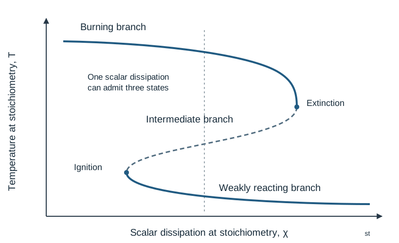
Fig. 14.1.3.1 Schematic steady diffusion-flame response. Multiple temperatures can occur at the same scalar dissipation. A suitable progress variable distinguishes reaction states within the retained flame family. The curve is qualitative.

The flamelet/progress-variable approach uses a reaction progress variable to distinguish these states [PM04]. Define \(C\) as a weighted sum of species mass fractions plus a constant:

(14.1.3.1)\[C=C_{\mathrm{off}}+\sum_{k=1}^{N_s}w_kY_k\]

Here \(N_s\) is the number of species. The weights \(w_k\) and offset \(C_{\mathrm{off}}\) are fixed, dimensionless constants for a given table. They are selected so that \(C\) distinguishes its chemical states. The weights can include a constant rescaling. Multiply each species equation by \(w_k\) and sum over species. Since the weights and offset are constant, \(\sum_k w_k\nabla Y_k=\nabla C\) and the result is

(14.1.3.2)\[\rho\frac{D C}{D t} =\nabla\cdot(\rho D\nabla C) +\sum_{k=1}^{N_s}w_k\dot\omega_k\]

The offset has zero material derivative. In conservative form, its contribution vanishes by continuity. Define the chemical source per unit mass as

(14.1.3.3)\[s_C^{\mathrm{chem}}=\frac{1}{\rho} \sum_{k=1}^{N_s}w_k\dot\omega_k\]

The specific source \(s_C^{\mathrm{chem}}\) has units of \(\mathrm{s}^{-1}\). The corresponding volumetric source in Eq. (14.1.3.2) is \(\rho s_C^{\mathrm{chem}}\).

The local value of \(C\) generally varies through a flamelet. A value such as \(C(Z_{\mathrm{st}})\) can label the entire reference solution, but that label is distinct from the local progress variable transported by the flow solver. Expressing the selected flamelet solutions in terms of \(Z\) and \(C\) gives the table relations

(14.1.3.4)\[Y_k=\mathcal Y_k(Z,C) \qquad s_{C,0}=s_{C,0}(Z,C)\]

The table stores \(s_{C,0}\), the value of \(s_C^{\mathrm{chem}}\) at the reference flamelet conditions. The flow model uses a third quantity, \(s_C\), after applying the turbulence and any state corrections. Their roles are

Symbol	Meaning
\(s_C^{\mathrm{chem}}\)	Chemical source obtained from the species production rates
\(s_{C,0}\)	Specific source supplied by the reference table
\(s_C\)	Modeled specific source used in the flow equation; its volumetric contribution is \(\rho s_C\)

The table requires a unique composition for each \((Z,C)\). The chosen progress variable must therefore distinguish the selected flamelet states.

Note

A progress variable need not equal one at equilibrium. Its range depends on its species weights and scaling. A mixture-dependent normalization, such as division by an equilibrium value that varies with \(Z\), introduces additional chain-rule terms in its transport equation. The simple progress equation developed here uses the constant coefficients in Eq. (14.1.3.1).

14.2. Flamelet Tabulation

The table is constructed for a specified mechanism, feed compositions, feed temperatures, and reference pressure. A diffusion-flame library samples strained reaction–diffusion states; a premixed-flame library samples a different balance involving flame propagation. Both can be parameterized by \(Z\) and \(C\), but their compositions and rates need not agree at the same coordinates.

The table supplies the mappings in Eq. (14.1.3.4), together with reference properties needed by the transport and source models. These may include reference temperature \(T_0\), reference density \(\rho_0\), molecular viscosity \(\mu_0\), thermal conductivity \(\lambda_0\), and coefficients describing temperature dependence. Reference properties can vary with \((Z,C)\) even when the reference pressure is fixed.

For a rectangular grid in \((Z,C)\), let \(Z_i\leq Z\leq Z_{i+1}\) and \(C_j\leq C\leq C_{j+1}\), and define

(14.2.1)\[\theta_Z=\frac{Z-Z_i}{Z_{i+1}-Z_i} \qquad \theta_C=\frac{C-C_j}{C_{j+1}-C_j}\]

A tabulated quantity \(f\) is recovered by bilinear interpolation:

(14.2.2)\[\begin{split}\begin{aligned} f(Z,C)={}&(1-\theta_Z)(1-\theta_C)f_{i,j} +\theta_Z(1-\theta_C)f_{i+1,j} \\ &+(1-\theta_Z)\theta_C f_{i,j+1} +\theta_Z\theta_C f_{i+1,j+1} \end{aligned}\end{split}\]

Within a table cell the weights are nonnegative and sum to one. Thus, if every tabulated composition is nonnegative and sums to one, applying the same weights to every species preserves those properties up to roundoff. Interpolation can still smooth sharp chemical variations, and it does not necessarily preserve nonlinear thermodynamic identities.

The coordinate rectangle is also distinct from the domain sampled by the reference flames. At a particular \(Z\), the flame family may cover only part of the available \(C\) interval. Values assigned outside that interval are extensions of the data, not additional flame solutions. Endpoint clamping similarly prevents extrapolation of the interpolation weights but does not establish physical validity outside the table range.

14.3. Transport Equations

14.3.1. Averaging and Scalar Closure

For turbulent flow, an overbar denotes a Reynolds average or an LES filter, as appropriate. The corresponding Favre quantity is

(14.3.1.1)\[\widetilde\phi=\frac{\overline{\rho\phi}}{\bar\rho}\]

Before closing the chemical source, the progress equation contains \(\overline{\rho s_C^{\mathrm{chem}}}\). This average generally differs from density multiplied by a chemical rate evaluated at the averaged state. Presumed probability-density-function (PDF) methods model the source by integrating over a distribution of reference states. The thickened-flame formulation uses the local modeled scalars and the source multiplier derived in Thickened Flame Closure.

The remaining flow equations omit bars and tildes. Density \(\rho\) and pressure \(p\) denote Reynolds means or filtered values; \(\vec u\), \(Z\), and \(C\) denote the corresponding Favre quantities. Temperature, composition, and thermodynamic properties are evaluated at the modeled local state. Unresolved scalar fluxes use gradient diffusion. For laminar flow, the same equations apply to instantaneous quantities with \(\mu_t=0\).

For flow without external mass sources, the modeled scalar balances are

(14.3.1.2)\[\frac{\partial(\rho Z)}{\partial t} +\nabla\cdot(\rho\vec u Z) =\nabla\cdot(\Gamma_Z\nabla Z)\]

(14.3.1.3)\[\frac{\partial(\rho C)}{\partial t} +\nabla\cdot(\rho\vec u C) =\nabla\cdot(\Gamma_C\nabla C)+\rho s_C\]

The term \(\rho s_C\) is the modeled volumetric source. The diffusion coefficients \(\Gamma_Z\) and \(\Gamma_C\) include density and have units of \(\mathrm{kg\,m^{-1}\,s^{-1}}\):

(14.3.1.4)\[\Gamma_Z=\Gamma_C=\rho D+\frac{\mu_t}{Sc_t} \qquad \rho D=\frac{\lambda}{c_p}\]

The molecular relation follows from a unity Lewis number, \(Le=\lambda/(\rho c_pD)=1\). The turbulent Schmidt number \(Sc_t\) relates eddy viscosity \(\mu_t\) to modeled scalar diffusion. These are separate assumptions: unity molecular Lewis number does not prescribe \(Sc_t\).

14.3.2. Total Energy and Enthalpy Diffusion

The specific internal energy \(e\) and static enthalpy \(h\) describe the modeled thermodynamic state. Specific total energy \(E\) and total enthalpy \(H\) include the kinetic energy of the mean or resolved velocity:

(14.3.2.1)\[E=e+\frac12|\vec u|^2 \qquad h=e+\frac{p}{\rho} \qquad H=E+\frac{p}{\rho}\]

For turbulent flow, these definitions omit a separate unresolved kinetic-energy contribution. Its transport flux is also omitted from the energy balance below. Turbulent enthalpy transport and stress work are retained through modeled fluxes. The additional correlations that arise from exact averaging are developed in RANS-Based Turbulence Models.

With these approximations, the modeled total-energy balance is

(14.3.2.2)\[\frac{\partial(\rho E)}{\partial t} +\nabla\cdot(\rho\vec u H) =-\nabla\cdot\vec q_{\mathrm{model}} +\nabla\cdot(\Matrix{\tau}_{\mathrm{eff}}\cdot\vec u)\]

The retained stress work uses the molecular and eddy viscosities through \(\Matrix{\tau}_{\mathrm{eff}}\). External heat and mechanical sources can be added in the form already defined in Governing Equations and Closure Structure. The flamelet-specific issue is how the energy flux and chemical composition are closed.

For an ideal-gas mixture, \(h=\sum_kY_kh_k(T)\), so

(14.3.2.3)\[\nabla h=c_p\nabla T+\sum_kh_k\nabla Y_k\]

Combining Fourier conduction with species diffusion \(\vec J_k=-\rho D\nabla Y_k\) gives

(14.3.2.4)\[\begin{split}\begin{aligned} \vec q &=-\lambda\nabla T+\sum_kh_k\vec J_k \\ &=-\lambda\nabla T-\rho D\sum_kh_k\nabla Y_k =-\rho D\nabla h \end{aligned}\end{split}\]

The last equality uses \(\rho D=\lambda/c_p\). This explains why a single enthalpy-gradient flux can carry both thermal and composition enthalpy. The adopted extension to the modeled flow is

(14.3.2.5)\[\vec q_{\mathrm{model}}=-\Gamma_h\nabla h \qquad \Gamma_h=\frac{\lambda}{c_p}+\frac{\mu_t}{Pr_t}\]

The turbulent enthalpy and scalar diffusivities coincide when \(Pr_t=Sc_t\). Using different turbulent Prandtl and Schmidt numbers changes that common-diffusivity approximation.

For a real-fluid mixture, enthalpy can also depend on pressure, and composition derivatives involve partial species enthalpies. Therefore Eq. (14.3.2.3) is not a general real-fluid identity. Equation (14.3.2.5) is retained as a modeled combined flux. It should not be supplemented with another species-enthalpy diffusion flux representing the same transport.

Chemical formation energy is included in \(e\) and \(h\). Reactions change \(C\) and therefore the recovered species composition. Thermodynamic recovery then converts that change, together with the transported energy, into a new temperature. Adding a separate chemical heat-release source to Eq. (14.3.2.2) would count formation-energy conversion twice. This is the same energy accounting developed in Reacting Flows with Finite-Rate Chemistry.

14.3.3. Molecular Transport Properties

Molecular viscosity and thermal conductivity are represented by local temperature power laws about the reference flamelet state:

(14.3.3.1)\[\mu=\mu_0\left(\frac{T}{T_0}\right)^{n_\mu} \qquad \lambda=\lambda_0\left(\frac{T}{T_0}\right)^{n_\lambda}\]

The reference values and exponents depend on \(Z\) and \(C\). The current \(T\) and \(c_p\) come from the energy and EOS calculation. These power laws model temperature dependence only; they provide no independent pressure or density correction to the transport properties.

14.4. Thickened Flame Closure

14.4.1. Thickening and Flame Efficiency

For a planar premixed reference flame, the elementary reaction–diffusion scalings are

(14.4.1.1)\[S_L\sim\sqrt{\frac{D}{\tau_{\mathrm{chem}}}} \qquad \delta_L\sim\sqrt{D\tau_{\mathrm{chem}}}\]

Here \(S_L\) is laminar flame speed and \(\delta_L\) is flame thickness. Let \(F\geq1\) be the thickening factor. Replacing \(D\) by \(FD\) and the reaction rate by \(s_{C,0}/F\) increases the chemical time to \(F\tau_{\mathrm{chem}}\). The ratio \(D/\tau_{\mathrm{chem}}\) is unchanged, while the product \(D\tau_{\mathrm{chem}}\) increases by \(F^2\). The scaling therefore preserves flame speed and increases thickness by \(F\). This permits a wider model flame to be represented on the flow mesh [CDVP00].

Thickening also changes how the flame interacts with unresolved motion. An efficiency factor \(\mathcal E\) accounts approximately for the associated change in flame surface and burning rate. The modeled diffusivity and source then have the factors

(14.4.1.2)\[D_{\mathrm{model}}=\mathcal E F D \qquad s_C=\frac{\mathcal E}{F}s_{C,0}\]

The planar flame scaling motivates this closure. Its application to strained or nonpremixed flames is an additional modeling assumption.

14.4.2. Algebraic Source Multiplier

An algebraic variant relates efficiency to thickening through [VAvO+08]

(14.4.2.1)\[\mathcal E=F^{\alpha_F}\]

The exponent \(\alpha_F\) describes the modeled wrinkling efficiency. The usual range discussed for this relation is \(0\leq\alpha_F\leq2/3\). The scalar equations already contain molecular and turbulent diffusion. To interpret that increased diffusion as flame thickening, form the ratio

(14.4.2.2)\[r_D=\frac{\mu/Sc_L+\mu_t/Sc_t}{\mu/Sc_L} =1+\frac{\mu_tSc_L}{\mu Sc_t}\]

The molecular Schmidt number \(Sc_L\) sets the molecular diffusion measure \(\mu/Sc_L\) used in this ratio. To match the scalar transport coefficient in Eq. (14.3.1.4), it must satisfy

(14.4.2.3)\[\frac{\mu}{Sc_L}=\frac{\lambda}{c_p} \qquad Sc_L=Pr_L \qquad Pr_L=\frac{\mu c_p}{\lambda}\]

Under this condition, \(r_D=\Gamma_C/(\rho D)\). Matching the thickened diffusivity \(\mathcal E F D\) to \(\Gamma_C/\rho\) therefore gives \(\mathcal E F=r_D\). Combining this relation with \(\mathcal E=F^{\alpha_F}\) gives

(14.4.2.4)\[F=r_D^{1/(1+\alpha_F)} \qquad \mathcal E=r_D^{\alpha_F/(1+\alpha_F)}\]

Their ratio is the source multiplier:

(14.4.2.5)\[G=\frac{\mathcal E}{F} =r_D^{(\alpha_F-1)/(\alpha_F+1)}\]

The baseline modeled progress source is therefore

(14.4.2.6)\[s_C=Gs_{C,0}(Z,C)\]

For nonnegative eddy viscosity and the stated exponent range, \(0<G\leq1\). Increasing eddy viscosity reduces \(G\); increasing \(\alpha_F\) at fixed \(r_D>1\) reduces this damping. As \(\mu_t\) tends to zero, \(r_D\) and \(G\) tend to one. The unmodified-source limit is also obtained by setting \(G=1\) independently of the eddy viscosity.

Important

The diffusion already present in the scalar equations supplies the thickening; no additional factor \(\mathcal E F\) is applied to it. If \(Sc_L\ne Pr_L\), the source multiplier remains a prescribed model, but \(r_D\) may differ from the actual total-to-molecular scalar diffusion ratio.

The diffusion ratio excludes numerical diffusion. Its eddy viscosity comes from the selected turbulence model, so RANS, LES, and hybrid models can produce different reaction rates.

14.5. Equation of State and Thermodynamic Recovery

14.5.1. Recovering the Thermodynamic State

The table supplies composition at \((Z,C)\), while the flow solution supplies pressure and total energy. First remove kinetic energy:

(14.5.1.1)\[e=E-\frac12|\vec u|^2\]

Convert species mass fractions to mole fractions using molecular weights \(W_k\):

(14.5.1.2)\[W_{\mathrm{mix}}=\left(\sum_k\frac{Y_k}{W_k}\right)^{-1} \qquad X_k=\frac{W_{\mathrm{mix}} Y_k}{W_k}\]

Here \(W_{\mathrm{mix}}\) is the mixture molecular weight. Hold composition fixed during thermodynamic recovery. The unknown temperature and molar volume must satisfy both the pressure EOS and the internal-energy relation at the supplied \(p\) and \(e\).

For a single-phase state, the pressure EOS determines volume at each trial temperature. The internal-energy relation, or caloric EOS, then supplies energy. The required temperature makes the energy residual zero:

(14.5.1.3)\[\mathcal R_e(T)=e_{\mathrm{EOS}}(p,T,X) -\left(E-\frac12|\vec u|^2\right)\]

Here \(X\) denotes the set of mole fractions. The pressure and caloric relations are developed below, followed by the recovery procedure and phase assumptions.

14.5.2. Peng–Robinson Mixture Equation

In molar units, the Peng–Robinson equation is [PR76]

(14.5.2.1)\[p=\frac{R_uT}{v_m-b} -\frac{a(T,X)}{v_m^2+2bv_m-b^2} \qquad \rho=\frac{W_{\mathrm{mix}}}{v_m}\]

Here \(R_u\) is the universal gas constant, \(v_m\) is molar volume, \(b\) is the mixture covolume, and \(a\) is the attraction parameter. The units of \(v_m\) and \(W_{\mathrm{mix}}\) must use the same mole basis. The mixture relations are

(14.5.2.2)\[a(T,X)=\sum_i\sum_jX_iX_ja_{ij}(T) \qquad b(X)=\sum_iX_ib_i\]

The critical-property correlations used to construct \(a_{ij}(T)\) and \(b_i\) are given in Mixture Parameters.

14.5.3. Caloric Properties and Departure Functions

Ideal-gas species enthalpies include their formation reference and temperature dependence:

(14.5.3.1)\[h_k^{\mathrm{ig}}(T) =h_k^{\mathrm{ig}}(T_{\mathrm{ref}}) +\int_{T_{\mathrm{ref}}}^{T}c_{p,k}^{\mathrm{ig}}(\vartheta)\,d\vartheta\]

The temperature-dependent functions are supplied by species NASA polynomial thermodynamics. The caloric reference \(T_{\mathrm{ref}}\) is distinct from the local flamelet reference temperature \(T_0\). Define molar ideal-gas mixture properties by

(14.5.3.2)\[h_m^{\mathrm{ig}}=\sum_kX_kW_kh_k^{\mathrm{ig}} \qquad c_{p,m}^{\mathrm{ig}}=\sum_kX_kW_kc_{p,k}^{\mathrm{ig}}\]

Departure functions give the difference from ideal-gas properties at the same temperature and composition. Write \(a_T=(\partial a/\partial T)_X\) and \(a_{TT}=(\partial^2a/\partial T^2)_X\), and define

(14.5.3.3)\[K=\frac{1}{2\sqrt2\,b} \ln\left[\frac{v_m+(1-\sqrt2)b}{v_m+(1+\sqrt2)b}\right]\]

The specific internal energy and enthalpy are

(14.5.3.4)\[e=\frac{h_m^{\mathrm{ig}}-R_uT+K(a-Ta_T)}{W_{\mathrm{mix}}} \qquad h=e+\frac{pv_m}{W_{\mathrm{mix}}}\]

The first two terms in the numerator give ideal-gas internal energy; \(K(a-Ta_T)\) is the nonideal correction. Both use molar units before division by \(W_{\mathrm{mix}}\). The attraction parameter and its derivatives are evaluated at the current temperature using Eqs. (14.5.2.2) and (14.5.6.2).

When all attraction and covolume contributions vanish, the model reduces to the ideal-gas mixture relations

(14.5.3.5)\[p=\rho\frac{R_u}{W_{\mathrm{mix}}}T \qquad e=\frac{h_m^{\mathrm{ig}}-R_uT}{W_{\mathrm{mix}}}\]

The ideal-gas limit is taken in the departure contribution as a whole; Eq. (14.5.3.3) is not evaluated by inserting \(b=0\) into its quotient.

14.5.4. Heat Capacities and Sound Speed

At fixed composition, the mass-specific heat capacities are defined by

(14.5.4.1)\[c_v=\left(\frac{\partial e}{\partial T}\right)_{v_m,X} \qquad c_p=\left(\frac{\partial h}{\partial T}\right)_{p,X}\]

The pressure derivatives at fixed composition follow directly from Eq. (14.5.2.1). With \(Q=v_m^2+2bv_m-b^2\),

(14.5.4.2)\[\begin{split}\begin{aligned} p_T\equiv\left(\frac{\partial p}{\partial T}\right)_{v_m,X} &=\frac{R_u}{v_m-b}-\frac{a_T}{Q} \\ p_v\equiv\left(\frac{\partial p}{\partial v_m}\right)_{T,X} &=-\frac{R_uT}{(v_m-b)^2}+\frac{2a(v_m+b)}{Q^2} \end{aligned}\end{split}\]

At fixed \(v_m\) and composition, \(K\) is independent of temperature. Differentiating the internal energy in Eq. (14.5.3.4) gives

(14.5.4.3)\[c_v=\frac{c_{p,m}^{\mathrm{ig}}-R_u-KTa_{TT}}{W_{\mathrm{mix}}}\]

For \(c_p\), volume changes with temperature while pressure stays fixed. Setting \(dp=p_T\,dT+p_v\,dv_m=0\) gives

(14.5.4.4)\[\left(\frac{\partial v_m}{\partial T}\right)_{p,X} =-\frac{p_T}{p_v}\]

The thermodynamic relation between the two heat capacities is

(14.5.4.5)\[c_p-c_v=\frac{T}{W_{\mathrm{mix}}} \left(\frac{\partial p}{\partial T}\right)_{v_m,X} \left(\frac{\partial v_m}{\partial T}\right)_{p,X}\]

Substituting the volume derivative gives

(14.5.4.6)\[c_p=c_v-\frac{T p_T^2}{W_{\mathrm{mix}} p_v}\]

For a stable single-phase state, define the isothermal compressibility \(\kappa_T\) and frozen-composition sound speed \(a_s\) by

(14.5.4.7)\[\kappa_T=-\frac{1}{v_m} \left(\frac{\partial v_m}{\partial p}\right)_{T,X} \qquad a_s^2=\left(\frac{\partial p}{\partial\rho}\right)_{s,X}\]

Here \(s\) is specific entropy. Using the pressure derivative and the thermodynamic relation between isothermal and isentropic compressibility gives

(14.5.4.8)\[\kappa_T=-\frac{1}{v_m p_v} \qquad a_s^2=\frac{c_p}{\rho c_v\kappa_T}\]

Composition is held fixed during the acoustic perturbation. In a real fluid, \(c_p/c_v\) generally differs from \(\rho a_s^2/p\).

14.5.5. Temperature Recovery and Phase Assumptions

For a single-phase state, solve Eq. (14.5.1.3) at fixed pressure and composition. At each trial temperature, the pressure EOS supplies an admissible molar volume with \(v_m>b\), and the caloric EOS supplies internal energy. A bracketed secant iteration adjusts temperature until the residual is zero. Density and the remaining properties follow from that same state. This recovery allows compression, expansion, and heat transfer to change temperature independently of the tabulated \(T_0\).

A cubic EOS may have several volume roots below its critical region. The smaller and larger admissible roots describe liquid-like and vapor-like states. The subcritical construction uses a saturation temperature and saturated end states to select the appropriate branch. At fixed composition, the saturation temperature makes the molar Gibbs energies of these two roots equal at the prescribed pressure. Where the energy lies between the saturated liquid and vapor energies, the adopted homogeneous mixture treatment uses the vapor mass fraction

(14.5.5.1)\[q_v=\frac{e-e_\ell}{e_v-e_\ell} \qquad \frac1\rho=\frac{1-q_v}{\rho_\ell}+\frac{q_v}{\rho_v}\]

The subscripts \(\ell\) and \(v\) identify saturated liquid and vapor at the same pressure and temperature. Both phases are assumed to have the same species composition. Enthalpy and heat capacities are mass-weighted between these end states, and the adopted acoustic mixture relation is

(14.5.5.2)\[\frac{1}{\rho^2a_s^2} =\frac{1-q_v}{\rho_\ell^2a_{s,\ell}^2} +\frac{q_v}{\rho_v^2a_{s,v}^2}\]

This homogeneous mixture model assumes equal phase compositions and no slip. A general multicomponent phase-equilibrium calculation instead finds a separate composition in each phase. On the saturation curve, pressure and temperature alone do not determine \(q_v\); an energy or volume constraint is also required.

14.5.6. Mixture Parameters

The binary parameters are formed from corresponding critical properties, following the mixture construction used for high-pressure flamelet thermodynamics [HMB97, MBHI17]. Let \(T_{c,i}\), \(p_{c,i}\), \(v_{c,i}\), \(\zeta_{c,i}\), and \(\omega_i\) denote species critical temperature, pressure, molar volume, critical compressibility factor, and acentric factor. The binary properties are

(14.5.6.1)\[\begin{split}\begin{aligned} T_{c,ij}&=\sqrt{T_{c,i}T_{c,j}} \\ v_{c,ij}&=\frac18 \left(v_{c,i}^{1/3}+v_{c,j}^{1/3}\right)^3 \\ \zeta_{c,ij}&=\frac{\zeta_{c,i}+\zeta_{c,j}}2 \qquad \omega_{ij}=\frac{\omega_i+\omega_j}2 \\ p_{c,ij}&=\frac{\zeta_{c,ij}R_uT_{c,ij}}{v_{c,ij}} \end{aligned}\end{split}\]

The critical compressibility factor \(\zeta_{c,i}=p_{c,i}v_{c,i}/(R_uT_{c,i})\) is dimensionless. It differs from the isothermal compressibility \(\kappa_T\), which has units of inverse pressure. The binary attraction parameters and species covolumes are

(14.5.6.2)\[\begin{split}\begin{aligned} m_{ij}&=0.37464+1.54226\omega_{ij}-0.26992\omega_{ij}^2 \\ a_{ij}(T)&=0.457236\frac{R_u^2T_{c,ij}^2}{p_{c,ij}} \left[1+m_{ij}\left(1-\sqrt{\frac{T}{T_{c,ij}}}\right)\right]^2 \\ b_i&=0.077796\frac{R_uT_{c,i}}{p_{c,i}} \end{aligned}\end{split}\]

Species modeled as ideal contributors have zero covolume and no attraction contribution. They still contribute molecular weight and ideal-gas caloric properties. The accuracy of the mixture EOS depends on the critical-property data for its nonideal species.

14.5.7. Chemical Rates Away from the Reference State

The baseline source in Eq. (14.4.2.6) retains the chemical rate from the reference table. Recovering a different thermodynamic state does not automatically recompute that rate. An optional local correction represents density and temperature effects by

(14.5.7.1)\[s_C=G s_{C,0} \left(\frac{\rho}{\rho_0}\right)^{\alpha_\rho} \exp\left[-T_a\left(\frac1T-\frac1{T_0}\right)\right]\]

The dimensionless exponent \(\alpha_\rho\) and activation temperature \(T_a\) are prescribed calibration data, potentially varying over the table. They are distinct from the wrinkling exponent \(\alpha_F\). Setting both coefficients to zero recovers the baseline source. The correction changes the rate at the composition supplied by the table.

A separate reaction-freezing model suppresses the chemical source at temperatures at or below a threshold \(T_f\). This is a prescribed source cutoff, not a prediction of ignition temperature or extinction.

14.6. Coupling to the Pressure Based Method

The scalar, momentum, pressure, and energy equations describe one coupled flow. Their main thermochemical relations are

(14.6.1)\[\begin{split}\begin{aligned} Y_k&=\mathcal Y_k(Z,C) \\ e&=E-\tfrac12|\vec u|^2 \\ (p,e,\{Y_k\})&\longmapsto(T,\rho,h,c_p,c_v,a_s) \\ s_C&=s_C(Z,C,T,\rho,\mu_t) \end{aligned}\end{split}\]

Changing progress changes composition and caloric properties. Changing energy changes temperature and can change transport and the modeled reaction rate. Density changes feed back into continuity and the face mass fluxes. Nonlinear iteration brings these quantities into agreement at the new physical time level; the pressure-correction development is given in Pressure-Correction Equation on Unstructured Grids.

For either scalar \(\phi\in\{Z,C\}\), integrate its transport equation over a fixed cell \(P\) of volume \(\Omega_P\). The divergence theorem converts the convective and diffusive terms to face integrals. Approximating the cell integrals with cell values and the face integrals with face values gives the balance

(14.6.2)\[\frac{d}{dt}\left[(\rho\phi)_P\Omega_P\right] +\sum_{f\in\mathcal F_P}\sigma_{Pf}\dot m_f\phi_f =\sum_{f\in\mathcal F_P}\sigma_{Pf} \Gamma_{\phi,f}(\nabla\phi)_f\cdot\vec A_f +(\rho s_\phi)_P\Omega_P\]

Here \(\mathcal F_P\) is the set of faces of cell \(P\), \(s_Z=0\), and \(s_C\) is the modeled progress source. The face mass flux \(\dot m_f\) and area vector \(\vec A_f\) use the guide’s stored face orientation. The incidence sign \(\sigma_{Pf}\) converts that orientation to an outward contribution for cell \(P\). The balance is discrete in space and continuous in time. Face approximations and time integration are developed in Finite-Volume Transport Assembly on Unstructured Grids and Higher-Order Temporal Integration and Splitting. The scalar equations must use mass fluxes consistent with continuity.

The same consistency is required when prescribing an initial or boundary state. Given \(p\), \(T\), \(Z\), and \(C\), composition comes from the table and the EOS determines density and internal energy. Total energy then includes the prescribed kinetic energy. Independently assigning all of these quantities can overdetermine the thermodynamic state.

Limiting transported scalars changes the cell state; clamping a table query only restricts the lookup. A nonconservative change to \(C\) also changes composition and the temperature recovered from the transported energy.

The optional double-flux treatment for coupling energy and pressure across strong property variations is developed in Double-Flux Method for a Pressure-Based Segregated Solver.

14.7. Assumptions and Limitations

The reference flames and closures determine the model’s range of use. The main assumptions and their consequences are collected below.

Assumption or approximation	Consequence
Two composition coordinates	Independent species histories, slow intermediates, and pollutants may require more coordinates or species equations.
Specified feeds and reference conditions	Changes in pressure, feed temperature, or dilution can require a different chemical table.
Steady reference flames, where used	Transient ignition and extinction can depend on chemical history absent from the table.
Common molecular diffusivity	The scalar equations omit preferential diffusion and nonunity-Lewis effects.
Algebraic thickening and efficiency	Burning depends on the turbulence and wrinkling models. Numerical diffusion and mesh or time resolution also affect the balance.
No heat-loss coordinate	Wall cooling changes temperature without a corresponding heat-loss-dependent composition.
Finite table coverage and resolution	Missing branches, nonunique mappings, interpolation, and data extensions limit the represented states.
Cubic mixture EOS and equal phase compositions	Accuracy depends on species data and mixture assumptions; general multicomponent phase separation is outside this closure.

An independently varying third feed requires another composition coordinate. Droplet evaporation, liquid-phase reactions, and other multiphase exchange mechanisms require additional equations and coupling terms.

14.8. References

[CDVP00]

O. Colin, F. Ducros, D. Veynante, and T. Poinsot. A thickened flame model for large eddy simulations of turbulent premixed combustion. Physics of Fluids, 12(7):1843–1863, 2000. doi:10.1063/1.870436.

[HMB97]

K. G. Harstad, R. S. Miller, and J. Bellan. Efficient high-pressure state equations. AIChE Journal, 43(6):1605–1610, 1997. doi:10.1002/aic.690430624.

[MBHI17]

Peter C. Ma, Daniel T. Banuti, Jean-Pierre Hickey, and Matthias Ihme. Numerical framework for transcritical real-fluid reacting flow simulations using the flamelet progress variable approach. In 55th AIAA Aerospace Sciences Meeting, number AIAA 2017-0143. 2017. doi:10.2514/6.2017-0143.

[PR76]

Ding-Yu Peng and Donald B. Robinson. A new two-constant equation of state. Industrial & Engineering Chemistry Fundamentals, 15(1):59–64, 1976. doi:10.1021/i160057a011.

[Pet00]

Norbert Peters. Turbulent Combustion. Cambridge University Press, 2000. doi:10.1017/CBO9780511612701.

[PM04]

C. D. Pierce and P. Moin. Progress-variable approach for large-eddy simulation of non-premixed turbulent combustion. Journal of Fluid Mechanics, 504:73–97, 2004. doi:10.1017/S0022112004008213.

[TWI19]

Siddharth Thakur, Jeffrey Wright, and Matthias Ihme. Compressible flamelet model with thickened flame closure in an all-speed combustion solver. In AIAA Scitech 2019 Forum, number AIAA 2019-2143. 2019. doi:10.2514/6.2019-2143.

[TWN24]

Siddharth Thakur, Jeffrey Wright, and Christopher Neal. A compressible flamelet-based turbulent combustion modeling framework in an all-speed solver for rocket engines. In Twelfth International Conference on Computational Fluid Dynamics (ICCFD12), number ICCFD12-2024-C000102. Kobe, Japan, 2024. URL: https://iccfd.org/iccfd12/assets/pdf/papers/ICCFD12_Paper_5-D-03.pdf.

[VAvO+08]

A. W. Vreman, B. A. Albrecht, J. A. van Oijen, L. P. H. de Goey, and R. J. M. Bastiaans. Premixed and non-premixed generated manifolds in large-eddy simulation of Sandia flame D and F. Combustion and Flame, 153(3):394–416, 2008. doi:10.1016/j.combustflame.2008.01.009.