19. Porous Media

A porous screen or solid matrix resists fluid motion. When its pores are not resolved by the grid, this resistance is represented by a force in the momentum equation. The matrix is stationary; its resistance may be isotropic or depend on direction.

The resistance-only model modifies momentum. The thermal models also account for fluid volume fraction and heat stored in the matrix. Local thermal equilibrium (LTE) uses one temperature; local thermal nonequilibrium (LTNE) retains separate fluid and solid temperatures.

19.1. Resistance Law

The momentum equation with porous resistance is

(19.1.1)\[\frac{\partial(\rho\vec u)}{\partial t} +\nabla\cdot(\rho\vec u\otimes\vec u) =-\nabla p+\nabla\cdot\Matrix{\tau}+\vec S_b+\vec S_p\]

Here \(\vec S_b\) contains other body forces and \(\vec S_p\) is the porous force per unit volume. Pressure is \(p\), density is \(\rho\), and \(\Matrix{\tau}\) is viscous stress, as in Governing Equations and Closure Structure. The bulk, or superficial, velocity \(\vec u\) is based on the total flow area, including the solid fraction. The resistance coefficients must use this velocity convention.

An isotropic resistance acts opposite to the velocity:

(19.1.2)\[\vec S_p=-C\vec u \qquad C=C(\rho,\mu,\lVert\vec u\rVert)\geq0\]

The dynamic viscosity is \(\mu\). The coefficient \(C\) has units of kg/(m\(^3\) s). The force removes kinetic energy because \(\vec u\cdot\vec S_p=-C\lVert\vec u\rVert^2\leq0\). A Darcy–Forchheimer law combines viscous and inertial drag:

(19.1.3)\[C=\mu d+\tfrac12\rho f\lVert\vec u\rVert\]

For permeability \(K\), the viscous coefficient \(d=1/K\) has units of inverse area. The inertial coefficient \(f\) has units of inverse length. Both are nonnegative. In the alternative convention \(C=\mu/K+\rho\beta_{\mathrm F}\lVert\vec u\rVert\), the same law has \(f=2\beta_{\mathrm F}\).

For steady one-dimensional flow with constant velocity \(U\) and coefficient \(C\), pressure balances drag when \(dp/dx=-CU\). Across a layer of thickness \(L\), the Darcy–Forchheimer law gives

(19.1.4)\[p(0)-p(L)=LCU =L\left(\mu dU+\tfrac12\rho f|U|U\right)\]

The positions \(0\) and \(L\) remain fixed when flow reverses. Thus the pressure difference changes sign with \(U\).

19.1.1. Screen Correlations

Screen correlations specify the scalar coefficient \(C\) through empirical parameters. The Armour–Cannon–Cady (ACC) correlation gives [AC68, Cad73]

(19.1.1.1)\[C_{\mathrm{ACC}} =\frac{B}{B_{\mathrm{CFD}}}\frac{Q_{\mathrm{ACC}}}{\epsilon^2} \left(\alpha_{\mathrm{ACC}}\mu a_v^2 +\frac{\beta_{\mathrm{ACC}}\rho\lVert\vec u\rVert}{D_p}\right)\]

Here \(\epsilon\) is void fraction, \(a_v\) is screen surface area per unit volume, \(D_p\) is hydraulic pore diameter, and \(Q_{\mathrm{ACC}}\) is a tortuosity factor. The constants \(\alpha_{\mathrm{ACC}}\) and \(\beta_{\mathrm{ACC}}\) set the viscous and inertial resistance. The ratio \(B/B_{\mathrm{CFD}}\) accounts for the physical screen thickness relative to the thickness of the modeled region.

The numerically determined resistance (NDR) correlation retains only quadratic drag:

(19.1.1.2)\[C_{\mathrm{NDR}} =\frac{\rho K_q\lVert\vec u\rVert}{2\epsilon^2}\]

The fitted coefficient \(K_q\) has units of inverse length. Both correlations require parameters that give \(C\geq0\) and a positive void fraction.

19.2. Force on a Control Volume

Let \(P\) denote a cell of volume \(\Omega_P\), with center \(\vec x_P\). The force density \(\vec S_p\) has units of N/m\(^3\). Its integrated contribution \(\vec{\mathcal B}_{p,P}\), in N, follows the notation of Consistency with Momentum Source Terms:

(19.2.1)\[\vec{\mathcal B}_{p,P}=\int_{\Omega_P}\vec S_p\,d\Omega\]

19.2.1. Cell-Centered Approximation

Evaluating the force at the cell center gives

(19.2.1.1)\[\vec{\mathcal B}_{p,P}^{\mathrm{std}} =\Omega_P\vec S_{p,P} =-\Omega_PC_P\vec u_P\]

The coefficient \(\Omega_PC_P\) has units of kg/s and multiplies velocity to give force.

19.2.2. Conservative Face Assembly

Consider an internal face with \(P\) on its stored left side and \(N\) on its right. The face center is \(\vec x_f\). The area vector \(\vec A_f=A_f\hat{\vec n}_f\) points from \(P\) to \(N\). Approximate the force as constant on each segment from the cell center to the face center. Its line integral is

(19.2.2.1)\[L_f(\vec S_p) =\vec S_{p,P}\cdot(\vec x_f-\vec x_P) +\vec S_{p,N}\cdot(\vec x_N-\vec x_f)\]

This is the line estimate defined in Eq. (5.7.1.2). It has pressure units and estimates \(p_N-p_P\) when pressure balances resistance along the path.

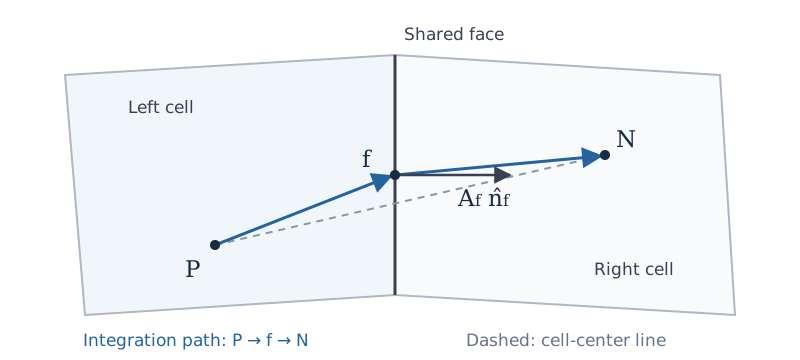
Fig. 19.2.2.1 The two segments used to estimate the pressure change due to resistance. The face center need not lie on the line joining the cell centers.

Use the distance weights from Eq. (5.4.1.11):

(19.2.2.2)\[w_N=\frac{\lVert\vec x_f-\vec x_P\rVert} {\lVert\vec x_f-\vec x_P\rVert+\lVert\vec x_N-\vec x_f\rVert} \qquad w_P=1-w_N\]

Ordinary interpolation is \(\mathcal I_f(q)=w_Pq_P+w_Nq_N\). For force assembly, multiply the pressure change by \(\vec A_f\) and distribute it in proportion to each cell’s segment length:

(19.2.2.3)\[\vec{\mathcal B}_{p,P\leftarrow f}^{\mathrm c} =w_N L_f(\vec S_p)\vec A_f \qquad \vec{\mathcal B}_{p,N\leftarrow f}^{\mathrm c} =w_P L_f(\vec S_p)\vec A_f\]

Cell \(P\) receives the fraction \(w_N\), which measures its own segment length. These weights therefore appear in the opposite order to ordinary interpolation. The shares sum to the entire force \(L_f(\vec S_p)\vec A_f\). Reversing the stored orientation reverses both \(L_f\) and \(\vec A_f\), leaving their product unchanged. Conversion to a cell-outward orientation likewise introduces two incidence signs, which cancel.

At a physical boundary, use the segment from the owner cell to the face and the outward area vector:

(19.2.2.4)\[\vec{\mathcal B}_{p,P\leftarrow f}^{\mathrm c} =\left[\vec S_{p,P}\cdot(\vec x_f-\vec x_P)\right]\vec A_f\]

Sum the contributions over the cell’s faces to obtain \(\vec{\mathcal B}_{p,P}^{\mathrm c}\). On a skewed mesh or across a change in resistance, this assembled force need not be parallel to \(-\vec u_P\), even for an isotropic material.

19.3. Explicit and Implicit Treatment

Here explicit and implicit refer to placement within the nonlinear momentum solve. Let \(k\) denote the current outer iteration and let a star mark the provisional velocity being solved. Evaluate \(C_P\) from the current state and hold it fixed during that solve.

With an explicit porous source, the unrelaxed momentum row is

(19.3.1)\[{}^{(u)}\!a_{P,0}\vec u_P^* =\sum_{N\in\mathcal N(P)}{}^{(u)}\!a_{P,N}\vec u_N^* +{}^{(u)}\!\vec b_{P,0} -\vec{\mathcal P}_P +\vec{\mathcal B}_{p,P}^{\,k}\]

The set \(\mathcal N(P)\) contains the neighboring cells. The diagonal \({}^{(u)}\!a_{P,0}\) excludes porous resistance, and \({}^{(u)}\!\vec b_{P,0}\) excludes both porous force and pressure. The pressure-gradient integral is \(\vec{\mathcal P}_P=\int_{\Omega_P}\nabla p\,d\Omega\); its force is \(-\vec{\mathcal P}_P\), following Eq. (5.3.7.1). The porous force uses either cell-centered or conservative assembly. All coefficients belong to iteration \(k\); those labels are suppressed.

For the cell-centered source, replace \(-\Omega_PC_P\vec u_P^k\) by \(-\Omega_PC_P\vec u_P^*\) and move it to the left:

(19.3.2)\[\left({}^{(u)}\!a_{P,0}+\Omega_PC_P\right)\vec u_P^* =\sum_{N\in\mathcal N(P)}{}^{(u)}\!a_{P,N}\vec u_N^* +{}^{(u)}\!\vec b_{P,0}-\vec{\mathcal P}_P\]

The positive addition \(\Omega_PC_P\) makes the drag respond to the velocity being solved. For conservative face assembly, the complete force can point in a different direction from \(-\vec u_P\). Retain the same local implicit term and evaluate the remainder from iteration \(k\):

(19.3.3)\[\vec{\mathcal B}_{p,P}(\vec u^*) \approx-\Omega_PC_P\vec u_P^* +\underbrace{\left(\vec{\mathcal B}_{p,P}^{\,k} +\Omega_PC_P\vec u_P^k\right)} _{\vec{\mathcal B}_{p,P}^{\,\mathrm{rhs},k}}\]

The remainder \(\vec{\mathcal B}_{p,P}^{\,\mathrm{rhs},k}\) is a known force on the right-hand side. Substitution gives

(19.3.4)\[\left({}^{(u)}\!a_{P,0}+\Omega_PC_P\right)\vec u_P^* =\sum_{N\in\mathcal N(P)}{}^{(u)}\!a_{P,N}\vec u_N^* +{}^{(u)}\!\vec b_{P,0}-\vec{\mathcal P}_P +\vec{\mathcal B}_{p,P}^{\,\mathrm{rhs},k}\]

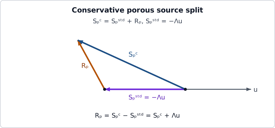
Fig. 19.3.1 Isotropic source split at a fixed iterate. The cell-centered contribution \(-\Omega_PC_P\vec u_P^k\) and the remainder sum to \(\vec{\mathcal B}_{p,P}^{\,\mathrm c,k}\). Cell and iteration indices are omitted in the diagram. The remainder need not be perpendicular to velocity; vector lengths are illustrative.

For cell-centered assembly the remainder is zero. For conservative assembly it preserves the part not represented by the local diagonal. At convergence, \(\vec u_P^*=\vec u_P^k\), and the split recovers the assembled force. Updating \(C_P\) between outer iterations is a Picard linearization of the speed-dependent resistance.

19.4. Face Flux and Pressure Correction

The face flux must include the pressure response of the momentum row and the same physical porous force. Use the face orientation and interpolation weights defined above, and let \(\ell_f=(\vec x_N-\vec x_P)\cdot\hat{\vec n}_f>0\) be the normal separation. The derivation below uses an orthogonal face and velocity relaxation \(0<\alpha_v\leq1\) applied to the complete momentum diagonal. Other body forces are omitted.

Denote that unrelaxed diagonal by \({}^{(u)}\!a_P\). It is \({}^{(u)}\!a_{P,0}\) for explicit treatment and \({}^{(u)}\!a_{P,0}+\Omega_PC_P\) for implicit treatment. The source contribution already present in the interpolated cell velocity is proportional to \(\mathcal I_f(\vec{\mathcal B}_p/{}^{(u)}\!a)\). Remove it and insert the face estimate \(L_f(\vec S_p)/\ell_f\), weighted by the same momentum coefficient as the face pressure gradient:

(19.4.1)\[\Delta\dot\Omega_{p,f} =\alpha_v A_f\left[ \mathcal I_f\left(\frac{\Omega}{{}^{(u)}\!a}\right) \frac{L_f(\vec S_p)}{\ell_f} -\mathcal I_f\left(\frac{\vec{\mathcal B}_p}{{}^{(u)}\!a}\right) \cdot\hat{\vec n}_f\right]\]

Use the physical force \(\vec{\mathcal B}_{p,P}\) in this correction. The remainder \(\vec{\mathcal B}_{p,P}^{\mathrm{rhs}}\) only belongs to the linearized cell equation.

Add the integrated-pressure correction from Eq. (5.7.1.5), with the same diagonal:

(19.4.2)\[\begin{split}\begin{aligned} \mathcal C_{p,f}^{\mathrm{int}}+\Delta\dot\Omega_{p,f} ={}&\alpha_v A_f \mathcal I_f\left(\frac{\vec{\mathcal P}-\vec{\mathcal B}_p} {{}^{(u)}\!a}\right)\cdot\hat{\vec n}_f \\ &-\alpha_v A_f\mathcal I_f\left(\frac{\Omega}{{}^{(u)}\!a}\right) \frac{(p_N-p_P)-L_f(\vec S_p)}{\ell_f} \end{aligned}\end{split}\]

The first term vanishes when pressure and porous force balance in each cell. The second vanishes when the pressure difference equals the line estimate. Both conditions are needed to preserve this balance at the face.

After these pressure and force corrections, the provisional volumetric flow rate is

(19.4.3)\[\begin{split}\begin{aligned} \dot\Omega_f^* ={}&A_f\mathcal I_f(\vec u^*)\cdot\hat{\vec n}_f +\mathcal C_{p,f}^{\mathrm{int}}+\Delta\dot\Omega_{p,f} \\ &+(1-\alpha_v)\left[\dot\Omega_f^k -A_f\mathcal I_f(\vec u^k)\cdot\hat{\vec n}_f\right] \end{aligned}\end{split}\]

Here \(\dot\Omega_f\) has units of m\(^3\)/s and is positive from the stored left cell to the right. The last term retains the previous iteration’s face-flux correction, as derived in Classical Rhie–Chow Form and Under-Relaxation. The mass flow rate is \(\dot m_f=\rho_f\dot\Omega_f\).

For time-consistent scalar interpolation, use Eq. (5.7.1.4) with \(\vec S=\vec S_p\) and \(\vec{\mathcal B}=\vec{\mathcal B}_p\). Its spatial diagonal includes any implicit porous resistance; the face denominator and history terms follow the selected interpolation.

19.5. Directional Resistance

For an anisotropic material, replace the scalar coefficient by a tensor:

(19.5.1)\[\vec S_p=-\Matrix{R}\vec u \qquad \Matrix{R}=\mu\Matrix{D}+\tfrac12\rho\lVert\vec u\rVert\Matrix{F}\]

The coefficients \(d_i\) and \(f_i\) specify viscous and inertial resistance along three mutually perpendicular material axes. With these unit axes as columns of \(\Matrix{Q}\),

(19.5.2)\[\begin{split}\begin{aligned} \Matrix{D}&=\Matrix{Q}\,\operatorname{diag}(d_1,d_2,d_3)\Matrix{Q}^T \\ \Matrix{F}&=\Matrix{Q}\,\operatorname{diag}(f_1,f_2,f_3)\Matrix{Q}^T \end{aligned}\end{split}\]

Both tensors share the same material axes. The \(d_i\) have units of inverse area and the \(f_i\) have units of inverse length. Nonnegative coefficients make \(\Matrix{R}\) symmetric positive semidefinite, so \(\vec u\cdot\vec S_p=-\vec u\cdot\Matrix{R}\vec u\leq0\). The force can change the flow direction while removing kinetic energy. Setting \(d_i=d\) and \(f_i=f\) gives the isotropic limit \(\Matrix{R}=C\Matrix{I}\), where \(\Matrix{I}\) is the identity tensor.

19.5.1. Momentum Row

Hold the tensor \(\Matrix{R}_P\) fixed at the current outer iteration. Replacing \(C_P\Matrix{I}\) by \(\Matrix{R}_P\) in the scalar source split gives the local momentum matrix

(19.5.1.1)\[\Matrix{A}_P={}^{(u)}\!a_{P,0}\Matrix{I}+\Omega_P\Matrix{R}_P\]

Its entries have units of kg/s. The deferred force is now \(\vec{\mathcal B}_{p,P}^{\,k}+\Omega_P\Matrix{R}_P\vec u_P^k\). Thus the implicit row has the same right-hand-side construction as Eq. (19.3.4), with \(\Matrix{A}_P\vec u_P^*\) on the left. The isotropic limit is \(\Matrix{A}_P=({}^{(u)}\!a_{P,0}+\Omega_PC_P)\Matrix{I}\).

For SIMPLE, neglect neighboring velocity corrections while holding the momentum coefficients fixed. With velocity relaxation applied to the complete matrix, an integrated pressure-gradient correction gives

(19.5.1.2)\[\frac{\Matrix{A}_P}{\alpha_v}\vec u'_P\approx-\vec{\mathcal P}'_P \qquad \vec u'_P\approx-\alpha_v\Matrix{A}_P^{-1}\vec{\mathcal P}'_P\]

19.5.2. Face Flux

Interpolate the cell inverse from Eq. (19.5.1.2), including cell volume, to obtain

(19.5.2.1)\[\Matrix{M}_f=\mathcal I_f\left(\alpha_v\Omega\Matrix{A}^{-1}\right) \qquad m_f=\hat{\vec n}_f\cdot\Matrix{M}_f\hat{\vec n}_f\]

The tensor \(\Matrix{M}_f\) converts a force per unit volume into a face velocity; \(m_f\) is its response in the normal direction. Both have units of m\(^3\) s/kg. Interpolate the cell inverses, not the cell matrices. A pressure gradient at the face contributes \(-A_f\hat{\vec n}_f\cdot\Matrix{M}_f\nabla p\) to volumetric flux. Let \(\vec r_{PN}=\vec x_N-\vec x_P\). Separate the face coefficient into a part along \(\vec r_{PN}\) and a remainder. Approximate \(\vec r_{PN}\cdot\nabla p\) by \(p_N-p_P\) and evaluate the remainder with the current interpolated gradient:

(19.5.2.2)\[\hat{\vec n}_f\cdot\Matrix{M}_f\nabla p \approx\frac{m_f}{\ell_f}(p_N-p_P) +\left(\Matrix{M}_f\hat{\vec n}_f-\frac{m_f}{\ell_f}\vec r_{PN}\right) \cdot\mathcal I_f(\nabla p)\]

Holding the cell predictor, source terms, pressure gradient, density, and momentum coefficients fixed, a pressure correction changes mass flux by

(19.5.2.3)\[\dot m'_f=-d_f(p'_N-p'_P) \qquad d_f=\rho_f A_f\frac{m_f}{\ell_f}\]

For positive density, cell volumes, and \({}^{(u)}\!a_{P,0}\), nonnegative principal resistance coefficients make \(\Matrix{A}_P\) positive definite. With positive interpolation weights and \(\ell_f>0\), this gives \(d_f>0\): increasing \(p_N-p_P\) reduces flux in the stored direction.

Removing the cell pressure contribution and inserting this face estimate gives the pressure term in Eq. (19.4.3):

(19.5.2.4)\[\begin{split}\begin{aligned} \mathcal C_{p,f}^{\mathrm{int}} ={}&A_f\hat{\vec n}_f\cdot \mathcal I_f\left(\alpha_v\Matrix{A}^{-1}\vec{\mathcal P}\right) -\frac{d_f}{\rho_f}(p_N-p_P) \\ &-A_f\left[\Matrix{M}_f\hat{\vec n}_f -\frac{m_f}{\ell_f}\vec r_{PN}\right]\cdot\mathcal I_f(\nabla p) \end{aligned}\end{split}\]

The last term accounts for directional resistance and mesh nonorthogonality. It is held fixed during pressure correction and updated with the pressure gradient at the next outer iteration.

For the porous force, use the segment weights to form \(\vec S_{p,f}=w_N\vec S_{p,P}+w_P\vec S_{p,N}\). On an orthogonal face, \(\vec S_{p,f}\cdot\hat{\vec n}_f=L_f(\vec S_p)/\ell_f\). On a skewed face, this weighted vector is a separate approximation to the face source. Applying the same tensor coefficient and removing the cell contribution gives

(19.5.2.5)\[\Delta\dot\Omega_{p,f} =A_f\hat{\vec n}_f\cdot \left[\Matrix{M}_f\vec S_{p,f} -\mathcal I_f\left(\alpha_v\Matrix{A}^{-1}\vec{\mathcal B}_p\right)\right]\]

For a constant force and a linear pressure field with \(\nabla p=\vec S_p\), the face terms cancel. If \(\vec{\mathcal P}_P=\vec{\mathcal B}_{p,P}\) in each cell as well, the total pressure–force correction is zero. The isotropic limit on an orthogonal face recovers Eq. (19.4.1).

19.6. Time Integration

Porous force belongs to the spatial momentum residual. Its time weighting and history terms follow the formulas in the time-integration chapter. For constant \(\rho>0\) and \(C>0\), the source-only equation \(\rho\,d\vec u/dt=-C\vec u\) has decay time \(\rho/C\). Thus \(C\Delta t/\rho\) measures how well the time step resolves drag decay. Implicit source treatment improves the nonlinear solve; temporal accuracy still requires resolving the motion of interest.

19.7. Local Thermal Equilibrium

Local thermal equilibrium (LTE) assumes that the fluid and solid share a temperature \(T\). It applies when heat exchange between them is fast compared with the resolved flow and heating times.

19.7.1. Model and Averaged Quantities

Consider a rigid, stationary matrix with porosity \(0<\epsilon\leq1\) fixed in time. The fluid has one species, and the flow is laminar. Resistance and thermal conductivity are isotropic; other body forces are omitted.

Let \(\vec v\) be intrinsic fluid velocity, averaged over the pore volume. The superficial velocity is \(\vec u=\epsilon\vec v\). Density \(\rho\) and specific enthalpy \(h\) are intrinsic fluid properties. Thus \(\epsilon\rho\) is fluid mass per total volume, while \(\rho\vec u\) is mass flux per total area. The mass and momentum balances are

(19.7.1.1)\[\begin{split}\begin{aligned} \frac{\partial(\epsilon\rho)}{\partial t} +\nabla\cdot(\rho\vec u)&=0 \\ \frac{\partial(\epsilon\rho\vec v)}{\partial t} +\nabla\cdot(\rho\vec u\otimes\vec v) &=-\epsilon\nabla p+\nabla\cdot\Matrix{\tau}_b-\epsilon C\vec u \end{aligned}\end{split}\]

The bulk viscous stress is approximated by \(\Matrix{\tau}_b=\epsilon\mu[\nabla\vec v+(\nabla\vec v)^T -\tfrac23(\nabla\cdot\vec v)\Matrix{I}]\). The coefficient \(C=C(\rho,\mu,\lVert\vec u\rVert)\) follows the Darcy–Forchheimer law in Eq. (19.1.3), using superficial velocity.

19.7.2. Combined Fluid–Solid Energy Balance

For constant solid density \(\rho_s\) and specific heat \(c_s\), the solid heat capacity per total volume is \(C_s=(1-\epsilon)\rho_s c_s\), in J/(m\(^3\) K). With a fixed energy reference, its stored energy is \(C_sT\). The fluid total enthalpy and total energy per unit mass are \(H=h+\tfrac12\lVert\vec v\rVert^2\) and \(E=H-p/\rho\). The combined stored energy per total volume is therefore

(19.7.2.1)\[\epsilon\rho E+C_sT=\epsilon(\rho H-p)+C_sT\]

Heat transferred between fluid and solid enters their energy balances with opposite signs. Adding those balances cancels this internal exchange. The stationary solid stores and conducts energy, while only the fluid advects enthalpy:

(19.7.2.2)\[\frac{\partial[\epsilon(\rho H-p)+C_sT]}{\partial t} +\nabla\cdot(\rho\vec uH) =\nabla\cdot\left(\lambda_{\mathrm{eff}}\nabla T +\Matrix{\tau}_b\cdot\vec v\right)+S_{\rho E}\]

Here \(\lambda_{\mathrm{eff}}\) is the combined material conductivity in W/(m K), with heat flux based on total area. The imposed source \(S_{\rho E}\) is heating per total volume in W/m\(^3\); a negative value removes heat. Both quantities already refer to the bulk material and receive no further porosity factor. Drag converts kinetic energy to internal energy within this combined system, so it supplies no additional total-energy source.

Since porosity is fixed in time, moving the pressure derivative to the right gives the total-enthalpy form:

(19.7.2.3)\[\frac{\partial(\epsilon\rho H+C_sT)}{\partial t} +\nabla\cdot(\rho\vec uH) =\epsilon\frac{\partial p}{\partial t} +\nabla\cdot\left(\lambda_{\mathrm{eff}}\nabla T +\Matrix{\tau}_b\cdot\vec v\right)+S_{\rho E}\]

This is one energy equation for the common temperature, expressed through fluid total enthalpy.

19.7.3. Thermodynamic Closure

At the current pressure and intrinsic velocity, recover temperature from \(h(p,T)=H-\tfrac12\lVert\vec v\rVert^2\), then evaluate \(\rho(p,T)\). Heating and pressure loss change density through this fluid EOS. Porosity weights the fluid inventory; the matrix heat capacity contributes to Eq. (19.7.2.3) without changing the fluid EOS properties.

The fluid specific heat \(c_p=(\partial h/\partial T)_p\) relates temperature and enthalpy changes at fixed pressure. In a sealed, rigid volume at rest, fluid density is instead fixed, and the heat capacity per total volume is \(\epsilon\rho c_v+C_s\), where \(e\) is specific internal energy and \(c_v=(\partial e/\partial T)_\rho\). In steady flow with no applied heating, conduction, or viscous work, \(H\) is constant along the flow. A real-fluid EOS can still give a temperature change as pressure falls.

19.7.4. Discrete Enthalpy Equation

Integrate Eq. (19.7.2.2) over a fixed cell of volume \(\Omega_P\) and approximate its inventory by the cell-center value:

(19.7.4.1)\[\mathcal E_P=\Omega_P\left[\epsilon(\rho H-p)+C_sT\right]_P\]

Let \(\mathcal F_{E,f}\) be the total energy flow through face \(f\) in its stored direction. It includes enthalpy transport, conductive heat flow, and viscous work. With \(n\) and \(n+1\) denoting consecutive physical time levels separated by \(\Delta t\), backward Euler gives

(19.7.4.2)\[\frac{\mathcal E_P^{n+1}-\mathcal E_P^n}{\Delta t} +\sum_f\sigma_{Pf}\mathcal F_{E,f}^{n+1} =\Omega_P S_{\rho E,P}^{n+1}\]

The incidence sign \(\sigma_{Pf}\) converts each stored face flow to the outward direction for cell \(P\), as defined in Loci Face Orientation and Cell Incidence. In particular, the solid contribution to the storage term is

(19.7.4.3)\[\frac{C_{s,P}\Omega_P}{\Delta t}(T_P^{n+1}-T_P^n)\]

At outer iteration \(k\), hold pressure and velocity fixed during the enthalpy solve. Linearizing the EOS temperature in \(H\) gives

(19.7.4.4)\[T_P^{k+1}\approx T_P^k+\frac{H_P^{k+1}-H_P^k}{c_{p,P}^k}\]

Substitute this expression into the solid-storage term. Collect the coefficient of \(H_P^{k+1}\) on the left and the known terms on the right:

(19.7.4.5)\[\begin{split}\begin{aligned} {}^{(H)}\!a_{P,\mathrm s} &=\frac{C_{s,P}\Omega_P}{c_{p,P}^k\Delta t} \\ {}^{(H)}\!b_{P,\mathrm s} &={}^{(H)}\!a_{P,\mathrm s}H_P^k -\frac{C_{s,P}\Omega_P}{\Delta t}(T_P^k-T_P^n) \end{aligned}\end{split}\]

Let \({}^{(H)}\!a_{P,0}\) and \({}^{(H)}\!b_{P,0}\) contain all other terms, including porosity-weighted fluid storage, transport, pressure work, and applied heating. The enthalpy row becomes

(19.7.4.6)\[\left({}^{(H)}\!a_{P,0}+{}^{(H)}\!a_{P,\mathrm s}\right)H_P^{k+1} =\sum_{N\in\mathcal N(P)}{}^{(H)}\!a_{P,N}H_N^{k+1} +{}^{(H)}\!b_{P,0}+{}^{(H)}\!b_{P,\mathrm s}\]

The EOS temperature and \(c_p\) are updated between outer iterations. At convergence, the added terms recover the solid energy change in Eq. (19.7.4.3).

19.7.5. Heat Conduction Between Cells

Consider an orthogonal face with cell \(P\) on its stored left side and \(N\) on its right. Let \(\ell_P\) and \(\ell_N\) be the center-to-face distances, and let \(\lambda_P\) and \(\lambda_N\) denote the effective conductivities. Assuming perfect thermal contact at the face and constant conductivity on each segment, the two thermal resistances add. The conductive heat flow, positive from \(P\) to \(N\), is

(19.7.5.1)\[\dot Q_f=\frac{A_f(T_P-T_N)} {\ell_P/\lambda_P+\ell_N/\lambda_N}\]

The interface temperature is continuous, while its normal gradient changes to carry the same heat flow through both materials. If either conductivity is zero, the series resistance gives zero heat flow. For a nonorthogonal face, use the temperature-gradient correction in Eq. (4.2.1.16), with face conductivity obtained from the same two segment resistances.

The full face energy flow in Eq. (19.7.4.2) is

(19.7.5.2)\[\mathcal F_{E,f}=\dot m_fH_f+\dot Q_f -\left(\Matrix{\tau}_b\cdot\vec v\right)_f\cdot\vec A_f \qquad \dot m_f=\rho_f\vec u_f\cdot\vec A_f\]

Each internal face has one flow rate and opposite incidence signs in its two cell balances, so its contributions cancel when those balances are summed.

19.7.6. Pressure and Velocity Coupling

All convected quantities use the same mass flow \(\dot m_f\). Interpolate \(\epsilon\vec v\) to form the cell part of the superficial face velocity. For SIMPLE, hold the momentum coefficients fixed and neglect neighboring velocity corrections. The integrated pressure force then gives

(19.7.6.1)\[\vec v'_P\approx -\frac{\alpha_v\epsilon_P\Omega_P}{{}^{(v)}\!a_P}(\nabla p')_P \qquad \vec u'_P=\epsilon_P\vec v'_P\]

Here \({}^{(v)}\!a_P\) is the complete unrelaxed momentum diagonal, including the drag contribution \(\epsilon_P^2 C_P\Omega_P\), and \(\alpha_v\) is velocity relaxation. One porosity factor comes from the pressure force and the other from converting intrinsic to superficial velocity. On an orthogonal face, interpolating this coefficient gives

(19.7.6.2)\[\dot m'_f=-d_f(p'_N-p'_P) \qquad d_f=\rho_f\alpha_v\frac{A_f}{\ell_f} \mathcal I_f\left(\frac{\epsilon^2\Omega}{{}^{(v)}\!a}\right)\]

The center-to-center distance is \(\ell_f=\ell_P+\ell_N\). This expression is the velocity-induced part of the mass-flow correction; density changes also enter the compressible continuity equation.

SIMPLEC approximates neighboring velocity corrections using the local correction, as in Eq. (5.9.5.2). The time and local drag terms remain in the resulting diagonal. Let \({}^{(v)}\!a_{P,\mathrm{time}}\) be the momentum time-discretization coefficient before relaxation. The cell response becomes

(19.7.6.3)\[\vec v'_P\approx -\frac{\alpha_v\epsilon_P\Omega_P} {(1-\alpha_v){}^{(v)}\!a_P +\alpha_v\left({}^{(v)}\!a_{P,\mathrm{time}} +\epsilon_P^2C_P\Omega_P\right)}(\nabla p')_P\]

The ratio of retained time and drag coefficients to the remaining spatial diagonal is

(19.7.6.4)\[\delta_P= \frac{{}^{(v)}\!a_{P,\mathrm{time}}+\epsilon_P^2C_P\Omega_P} {{}^{(v)}\!a_P-{}^{(v)}\!a_{P,\mathrm{time}}-\epsilon_P^2C_P\Omega_P}\]

With coefficients held fixed, Eq. (19.7.6.3) is the SIMPLE response multiplied by \(1+\alpha_v/(1-\alpha_v+\delta_P)\). The face approximation interpolates \(\delta\) and applies the same form to the predictor coefficient \(d_f\):

(19.7.6.5)\[\dot m'_f=-\left(1+ \frac{\alpha_v}{1-\alpha_v+\mathcal I_f(\delta)}\right) d_f(p'_N-p'_P)\]

This is the interpolation approximation in Eq. (5.9.5.6). It requires a positive retained diagonal and a nonnegative spatial remainder. In the purely local limit, the remainder vanishes, \(\delta_P\) tends to infinity, and the multiplier tends to one. Keeping drag in the retained diagonal preserves the pressure response when resistance dominates transport.

For the local density correction, hold fluid \(H\) and \(\vec v\) fixed. Then \(dh=0\). Thermodynamic consistency gives

(19.7.6.6)\[\begin{split}\begin{aligned} \left(\frac{\partial h}{\partial p}\right)_T &=\frac{1}{\rho} +\frac{T}{\rho^2}\left(\frac{\partial\rho}{\partial T}\right)_p \\ dh&=c_p\,dT+\left(\frac{\partial h}{\partial p}\right)_T\,dp \end{aligned}\end{split}\]

Set \(dh=0\) in the second relation and substitute the resulting temperature change into the density differential:

(19.7.6.7)\[\begin{split}\begin{aligned} \rho'&\approx\left(\frac{\partial\rho}{\partial p}\right)_{H,\vec v}p' \\ \left(\frac{\partial\rho}{\partial p}\right)_{H,\vec v} &=\left(\frac{\partial\rho}{\partial p}\right)_T -\frac{1}{c_p}\left(\frac{\partial\rho}{\partial T}\right)_p \left(\frac{\partial h}{\partial p}\right)_T \end{aligned}\end{split}\]

This fixed-enthalpy derivative differs from the acoustic derivative in Density-Pressure Linearization In Pressure Correction. It describes the local pressure-correction step; the energy equation and EOS update the thermal state between outer iterations. In backward-Euler continuity, the density correction contributes \(\epsilon_P\Omega_P\rho'_P/\Delta t\) to fluid storage.

At an extrapolated-pressure boundary, include the pressure change associated with drag between the cell center and the face: \(\Delta p_f=-C_P\vec u_P\cdot(\vec x_f-\vec x_P)\). This follows from the local balance \(\nabla p=-C\vec u\) and preserves that balance when porous material reaches a prescribed-flow boundary.

19.8. Local Thermal Nonequilibrium

Local thermal nonequilibrium (LTNE) retains separate intrinsic fluid and solid temperatures, \(T_{\mathrm f}\) and \(T_{\mathrm s}\). The phase subscripts \(\mathrm f\) and \(\mathrm s\) distinguish these temperatures from a face value with subscript \(f\). The rigid-matrix assumptions and the mass and momentum balances in Eq. (19.7.1.1) still apply. Pore-scale interfaces are represented by distributed heat exchange within each porous cell.

19.8.1. Phase Energy Balances

Let \(H_v\geq0\) be the interphase heat-transfer coefficient per total volume, in W/(m\(^3\) K). It may represent the product of a surface heat-transfer coefficient and internal interfacial area per total volume. The exchange \(H_v(T_{\mathrm s}-T_{\mathrm f})\) heats the fluid when the solid is warmer and removes the same energy from the solid.

The effective phase conductivities \(\lambda_{\mathrm{f,eff}}\) and \(\lambda_{\mathrm{s,eff}}\) are in W/(m K), with conductive flux based on total area. Let \(S_{\mathrm f}\) and \(S_{\mathrm s}\) be imposed heating per total volume, in W/m\(^3\), positive into the respective phase. Using the solid heat capacity \(C_s\) and fluid total enthalpy \(H\) defined for LTE, the balances are

(19.8.1.1)\[\begin{split}\begin{aligned} \frac{\partial[\epsilon(\rho H-p)]}{\partial t} +\nabla\cdot(\rho\vec u H) &=\nabla\cdot(\lambda_{\mathrm{f,eff}}\nabla T_{\mathrm f} +\Matrix{\tau}_b\cdot\vec v) \\ &\quad+H_v(T_{\mathrm s}-T_{\mathrm f})+S_{\mathrm f} \\ C_s\frac{\partial T_{\mathrm s}}{\partial t} &=\nabla\cdot(\lambda_{\mathrm{s,eff}}\nabla T_{\mathrm s}) -H_v(T_{\mathrm s}-T_{\mathrm f})+S_{\mathrm s} \end{aligned}\end{split}\]

The stationary solid has no advective flux. Adding the equations cancels interphase exchange. The conductivities and source densities are already bulk quantities and receive no additional porosity factor. As in LTE, drag supplies no separate total-energy source.

Fluid and solid boundary heat fluxes belong to their respective equations. A prescribed fluid temperature does not prescribe the solid temperature. Where the solid ends at a free-fluid region, it can be insulated or exchange heat through the surface balance derived in Porous/Free-Fluid Interface.

19.8.2. Fluid Conductivity

A prescribed \(\lambda_{\mathrm{f,eff}}\) represents an effective fluid-phase conductivity per total area. A volume-fraction closure instead relates it to the intrinsic fluid conductivity \(\lambda_{\mathrm f}(T_{\mathrm f},p)\):

(19.8.2.1)\[\lambda_{\mathrm{f,eff}}=\epsilon\lambda_{\mathrm f}(T_{\mathrm f},p)\]

This isotropic closure accounts for the fluid fraction available for conduction. It contains no additional tortuosity or thermal-dispersion model. Outside the porous region, \(\epsilon=1\) and the intrinsic conductivity is recovered.

Between porous cells, each phase uses the series-resistance interpolation in Eq. (19.7.5.1), with its own effective conductivity on each side. The nonorthogonal correction uses the same face coefficient. A zero conductivity on either side blocks that conductive path. A coupled porous/free-fluid face instead uses the three connections described in Porous/Free-Fluid Interface.

For a prescribed outward fluid heat flux \(q_b\) in W/m\(^2\), the wall temperature is \(T_b=T_{\mathrm f,P}-q_b d_b/\lambda_{\mathrm{f,eff},P}\), where \(d_b\) is the normal cell-to-wall distance. The conductivity is evaluated at the adjacent cell state. Nonzero \(q_b\) requires positive conductivity. For a wall resistance \(R_b\) in m\(^2\) K/W connected to a reservoir at temperature \(T_r\), the same approximation gives

(19.8.2.2)\[q_b=\frac{T_{\mathrm f,P}-T_r} {d_b/\lambda_{\mathrm{f,eff},P}+R_b}\]

These expressions assume one-dimensional conduction between the cell center and wall. Prescribed-temperature walls evaluate conductivity at the boundary state. For temperature-dependent conductivity, both approximations resolve the local conductive resistance under mesh refinement.

19.8.3. Coupled Cell Equations

Integrate each phase balance over a cell of volume \(\Omega_P\). The fluid inventory and its face flows follow the LTE construction with the solid storage removed. The solid inventory is \(C_{s,P}\Omega_PT_{\mathrm s,P}\); its face flows contain only conduction. Each internal face flow enters the adjacent balances with opposite incidence signs, following Loci Face Orientation and Cell Incidence.

Use backward Euler for solid storage. At nonlinear iteration \(k\), hold pressure, velocity, and conductivities fixed during the coupled energy solve. Let \(\delta H_P\) and \(\delta T_{\mathrm s,P}\) be corrections to \(H_P^k\) and \(T_{\mathrm s,P}^k\). At fixed pressure and velocity, the fluid EOS gives \(\delta T_{\mathrm f,P}\approx\delta H_P/c_{p,P}^k\). The corresponding change in integrated exchange is

(19.8.3.1)\[\delta\!\left[H_v\Omega_P(T_{\mathrm s,P}-T_{\mathrm f,P})\right] \approx H_v\Omega_P\left(\delta T_{\mathrm s,P} -\frac{\delta H_P}{c_{p,P}^k}\right)\]

Let \({}^{(H)}\!a_{P,0}\) and \({}^{(T_{\mathrm s})}\!a_{P,0}\) be the fluid and solid diagonals before adding exchange, including any diagonal relaxation. Their units are kg/s and W/K, respectively. The neighbor coefficients \({}^{(H)}\!a_{P,N}\) and \({}^{(T_{\mathrm s})}\!a_{P,N}\) use the same right-hand-side convention as Eq. (19.7.4.6). Let \({}^{(H)}\!R_P^k\) and \({}^{(T_{\mathrm s})}\!R_P^k\) be the physical energy residuals in W: heating minus the rate of energy storage minus net outward energy flow. Heating includes the exchange term, with opposite signs in the two residuals.

For a cell away from the coupled porous/free-fluid surface, moving the exchange increments to the left gives the complete coupled row:

(19.8.3.2)\[\begin{split}\begin{aligned} \begin{bmatrix} {}^{(H)}\!a_{P,0}+H_v\Omega_P/c_{p,P}^k & -H_v\Omega_P \\ -H_v\Omega_P/c_{p,P}^k & {}^{(T_{\mathrm s})}\!a_{P,0}+H_v\Omega_P \end{bmatrix} \begin{bmatrix}\delta H_P\\\delta T_{\mathrm s,P}\end{bmatrix} &=\begin{bmatrix}{}^{(H)}\!R_P^k\\{}^{(T_{\mathrm s})}\!R_P^k\end{bmatrix} \\ &\quad+\sum_{N\in\mathcal N(P)} \begin{bmatrix} {}^{(H)}\!a_{P,N}\delta H_N\\ {}^{(T_{\mathrm s})}\!a_{P,N}\delta T_{\mathrm s,N} \end{bmatrix} \end{aligned}\end{split}\]

The fluid row couples to neighboring fluid enthalpies, and the solid row to neighboring solid temperatures. Volumetric exchange supplies the local cross terms. Its derivatives cancel when the two rows are added, just as its physical heat rates cancel in the summed energy balance.

Solve each local fluid–solid pair together within the spatial iteration. The complete spatial system must still converge. Relaxation acts on the transport and storage diagonals while retaining the full exchange block. If temperature bounds require damping, apply a common factor to both increments. Update temperature-dependent properties between nonlinear iterations and recompute both physical energy residuals on the accepted state; conductivity derivatives are omitted from the linear solve.

19.8.4. Porous/Free-Fluid Interface

At the edge of a porous region, fluid crosses an ordinary internal mesh face. Its shared mass flow transports enthalpy between porous and free fluid. No mass source is introduced at the face. The solid ends there, so its normal conductive flux requires a separate closure.

Consider a face of area \(A_f\) joining porous cell \(P\) and free-fluid cell \(N\). Here \(P\) identifies the porous side; either cell can be the stored left cell. Let \(\ell_P\) and \(\ell_N\) be positive normal distances from each cell center toward the face. The three temperatures are the pore fluid temperature \(T_{\mathrm f,P}\), solid temperature \(T_{\mathrm s,P}\), and free-fluid temperature \(T_N\).

For an orthogonal face, connect these temperatures to a common surface temperature \(T_\Gamma\). The conductances, in W/K, are

(19.8.4.1)\[\begin{split}\begin{aligned} G_{\mathrm f,P}&=\frac{A_f\lambda_{\mathrm{f,eff},P}}{\ell_P} \\ G_{\mathrm s,P}&=\frac{A_f} {\ell_P/\lambda_{\mathrm{s,eff},P}+R_\Gamma} \\ G_N&=\frac{A_f\lambda_N}{\ell_N} \end{aligned}\end{split}\]

Here \(\lambda_N\) is the free-fluid conductivity and \(R_\Gamma\geq0\) is an additional resistance between the solid and surface, in m\(^2\) K/W. Zero resistance gives perfect thermal contact. Each effective conductivity and the resistance refer to total face area. A zero conductivity gives zero conductance for that connection.

Assume the surface stores no energy. The sum of heat rates into it is zero:

(19.8.4.2)\[G_{\mathrm f,P}(T_{\mathrm f,P}-T_\Gamma) +G_{\mathrm s,P}(T_{\mathrm s,P}-T_\Gamma) +G_N(T_N-T_\Gamma)=0\]

Solve this balance for \(T_\Gamma\) and substitute it into each heat rate. For any two distinct connections \(i\) and \(j\), the resulting transfer from \(i\) to \(j\) is

(19.8.4.3)\[\dot Q_{i\to j}= \frac{G_iG_j}{G_{\mathrm f,P}+G_{\mathrm s,P}+G_N}(T_i-T_j)\]

The indices select the pore fluid, solid, or free fluid, with their conductances and temperatures defined above. Each transfer is removed from one balance and added to the other. The three cell energy balances therefore conserve interface heat. The pore-fluid/free-fluid transfer replaces the ordinary two-cell conductive flux at this face. The other two transfers add local pore-fluid/solid coupling in \(P\) and cross-phase coupling between the solid in \(P\) and fluid in \(N\) to Eq. (19.8.3.2).

For a nonorthogonal face, reconstruct each temperature along the tangential part of its center-to-face displacement. For the pore fluid, for example, replace \(T_{\mathrm f,P}\) in the heat rates by

(19.8.4.4)\[T_{\mathrm f,P}+(\nabla T_{\mathrm f})_P\cdot \left[(\vec x_f-\vec x_P) -\ell_P\sigma_{Pf}\hat{\vec n}_f\right]\]

Here \(\hat{\vec n}_f\) is the stored face normal and \(\ell_P=(\vec x_f-\vec x_P)\cdot\sigma_{Pf}\hat{\vec n}_f\). Use the solid gradient for the solid connection and the corresponding cell-\(N\) quantities for the free-fluid connection. Hold these gradients fixed during the linear solve and update them between nonlinear iterations.

An insulated solid termination sets \(G_{\mathrm s,P}=0\), leaving the usual two-fluid series resistance. If all three conductances vanish, there is no conductive transfer. Surface exchange is independent of the volumetric coefficient \(H_v\): setting \(H_v=0\) does not remove heat transfer through a coupled surface.

19.8.5. Limiting Cases

When \(H_v=0\) and the solid has no coupled surface, the two phase energy equations decouple. When \(\epsilon=1\) and solid conduction, heating, and exchange vanish, the solid row is absent. As \(H_v\) increases, the phase temperatures approach one another. With compatible phase boundary conditions, adding their balances gives LTE with \(\lambda_{\mathrm{eff}}=\lambda_{\mathrm{f,eff}}+\lambda_{\mathrm{s,eff}}\) and \(S_{\rho E}=S_{\mathrm f}+S_{\mathrm s}\).

For a sealed, rigid, spatially uniform cell containing a calorically perfect ideal gas, density and \(c_v\) are constant. The fluid heat capacity per total volume is \(C_f=\epsilon\rho c_v\). With no imposed heating or boundary heat transfer, the temperature difference obeys

(19.8.5.1)\[\frac{d(T_{\mathrm s}-T_{\mathrm f})}{dt} =-H_v\left(\frac{1}{C_f}+\frac{1}{C_s}\right) (T_{\mathrm s}-T_{\mathrm f})\]

The conserved energy is \(C_fT_{\mathrm f}+C_sT_{\mathrm s}\). For constant \(H_v\), backward Euler multiplies the previous temperature difference by \([1+\Delta t H_v(1/C_f+1/C_s)]^{-1}\), preserving its sign. The use of \(c_v\) in this closed-cell balance is consistent with the fixed-pressure \(c_p\) derivative in the enthalpy update: the surrounding flow iteration also updates pressure and density.

19.9. References

[AC68]

James C. Armour and Joseph N. Cannon. Fluid flow through woven screens. AIChE Journal, 14(3):415–420, 1968. doi:10.1002/aic.690140315.

[Cad73]

E. C. Cady. Study of thermodynamic vent and screen baffle integration for orbital storage and transfer of liquid hydrogen. Technical Report NASA-CR-134482, McDonnell Douglas Astronautics Company, 1973. URL: https://ntrs.nasa.gov/citations/19730025004.