Appendix: Thermodynamic Data

Thermodynamic properties for the fluid components involved in a simulation are specified in a chemistry model file. By convention, this file has the .mdl extension. To specify the model file for the simulation, use the run control file variable chemistry model in a manner:

chemistry_model: air_5s17r

The code will look for the file air_5s17r.mdl. By default, the code first looks in the directory from which the simulation was initiated. If the file is not found in this location, the code will attempt to look in the location defined by the environment variable CHEMISTRY_DATABASE, if defined, which contains several chemistry models for commonly used mixtures. If the file is not found in this location, the code will terminate with an error condition. The chemistry model file is divided into two sections. The first section contains the thermodynamic data for each of the species involved in the simulation. The second section contains a list of the chemical reactions among the species. Information in the species section is always required, while the reaction section may be left empty for non-combusting flow simulations. In this section, we describe the contents of the species section in detail. A parser-level format reference for both species and reactions is also provided below, with additional reaction-model discussion in the section devoted to simulations with finite rate chemistry.

The species section contains the complete thermodynamic specification for each species in the simulation. In the following, we first discuss the basic structure of the species section, followed by a parser-level reference for .mdl syntax (including reactions), and then practical workflows for generating model files. The thermal equation of state for all species is the ideal-gas law. Non-ideal-gas equations of state can be used by loading the real-fluids module. This is discussed in the final section.

Species Definition

The definitions for all species in the simulation are contained within a single species={}; block within the model file. An example of this section from the database model file air_5s17r.mdl looks as follows:

Example of a species section in a model file

species = {
   O2: <mf = 0.22> ;
   N2: <mf = 0.78> ;
   NO ;
   O ;
   N ;
   } ;

In this example, the file is declaring that there are five species in the simulation. Note that there is a minimum amount of information required to define the species in this case since most information for the species can be derived from pre-existing information in the species database. There are two distinct ways in which entries in the species section are interpreted by the code. If the species name is followed by an = character, then any information in the system database concerning this species is ignored.

The line below will specify the molecular mass, reference enthalpy, reference entropy, reference temperature, reference pressure and default mass fraction for the species H2, and over-ride any pre-existing information for this species in the database:

H2=<m=2.016, href=55749, sref=130751, Tref=300, Pref=101325, mf=1> ;

On the other hand, if the species name is followed by a : character, then the data specified is interpreted as augmenting the pre-existing data for that species. For example, the following line will augment the currently existing information for the species H2 with a polynomial definition for the specific heat over the temperature range 75K to 300K:

Augmenting the existing information for the species H2

H2:<cp=[75.0,poly(40.4475, -3.01156e-01, 2.35251e-03, -7.42018e-06, 8.35504e-09), 300.0]>

Multiple definition lines for a species can be present in the species section. For example, the complete definition for the species H2 could look as follows:

Complete definition for the species H2

H2=<m=2.016> ;
H2:<href=55749, sref=130751, Tref=300, Pref=101325, mf=1> ;
H2:<cp=[75.0,poly(40.4475, -3.01156e-01, 2.35251e-03, -7.42018e-06, 8.35504e-09), 300.0]>

Regardless of how the species are chosen to be defined, whether using the existing information in the species database and augmenting with additional data, or defining the species from scratch, it is important that all required thermodynamic variable are defined. The table below lists the variables that are used to specify the thermodynamic properties for each species.

Variables for Species Thermodynamic Definition

Variable	Description	Units	Notes
m	Molecular Mass	amu	Automatically generated from database
n	Linear component of \(e(T)\)	–	Used in vibrational equilibrium model
theta_v	Vibrational Temperature	\(K\)	Used in vibrational equilibrium model
href	Reference Enthalpy	\(\frac {J}{Kmol}\)	Used to compute \(K_{C}\)
sref	Reference Entropy	\(\frac {J}{(Kmol \cdot K)}\)	Used to compute \(K_{C}\)
Tref	Reference Temperature	\(K\)	Used to compute various thermodynamic properties
Pref	Reference Pressure	Pa	Used to compute \(K_{C}\)
mf	Mass Fraction	–	Not used
cp	Curve Fit for Specific Heat	\(\frac {J}{(Kmol \cdot K)}\)	Vibration equilibrium used outside range

MDL File Syntax and Format Reference

This section summarizes the format accepted by Stream’s .mdl parser.

Top-level structure:

Top-level MDL block layout

species = {
   ...
} ;

reactions = {
   ...
} ;

// Optional cgs units for reaction rate constants:
reactions(cgs) = {
   ...
} ;

General parser rules:

• Whitespace is ignored.

• // comments are supported.

• Every species/reaction statement must end with ;.

• The species={...} and reactions={...} blocks must also end with ;.

Species entry forms:

Species statement forms

species = {
   O2 ;                    // use database/default entry
   O2 = <...> ;            // replace existing entry
   O2 : <...> ;            // reuse existing entry, then override/add fields
} ;

Reaction entry forms:

Reaction statement forms

reactions = {
   O2 + O <-> 2 O2 ;             // use default reaction option data if available
   O2 + O <-> 2 O2 = <...> ;     // set reaction options
   O2 + O <-> 2 O2 : <...> ;     // reuse existing/default options then override
} ;

Reaction-equation syntax:

Reaction equation syntax

[nu]A + [nu]B <-> [nu]C + [nu]D
[nu]A + [nu]B ->  [nu]C + [nu]D

Notes:

• nu is an optional real stoichiometric coefficient (for example 0.5O2).

• M can be used as a third-body species in the reaction equation.

• Charged species suffixes (+) and (-) are supported in names.

• (s) markers are accepted in reaction expressions.

Option block and value syntax:

Options syntax used in species/reaction statements

<key=value, key2=value2, key3, key4=$false, key5="text">

Allowed value forms:

• real numbers (for example 3.14)

• real numbers with units (for example 3.3e4cal/mol)

• names (for example Thermodynamic)

• strings (for example "N(+)")

• functions (for example Arrhenius(C=1e12,eta=0,Ea=3.3e4cal/mol))

• lists (for example [A=1.0, B=2.0])

• booleans ($true / $false) or implicit true via key-only entries

Species option keys recognized by the parser:

• m

• n

• gamma

• theta_v

• mf

• href

• sref

• Tref

• Pref

• cp

• eos

• q

Reaction option keys recognized by the parser:

• Kf

• Kc

• MB

• exp_nu

• rate_modifier

• MinMF

• Troe

• Low

• High

Common reaction option patterns:

Typical reaction option patterns

Kf = Arrhenius(C=2e12, eta=0, Ea=3.3e4cal/mol)
Kc = Thermodynamic
MB = [H2=2.5, H2O=16.25, "N(+)"=4.29]
Low = Arrhenius(...)
High = Arrhenius(...)
Troe = [alpha=0.7346, Tsss=94, Ts=1756, Tss=5182]
exp_nu = [Fuel=0.5, O2=1.0]
rate_modifier = pressure(0.3, 1.01325e5)
rate_modifier = Rox(...)

Reaction-rate fit definitions:

The Arrhenius form used in Kf (and optionally Kc) is:

\[k_f(T) = C T^{\eta} \exp\left(-\frac{\theta}{T}\right)\]

In .mdl syntax this can be written either positionally, such as Arrhenius(C, eta, theta), or with named arguments, such as Arrhenius(C=2e12, eta=0, Ea=3.3e4cal/mol).

For concentration-unit conventions:

• reactions={...} uses SI concentration reference (\(Kmol/m^3\)).

• reactions(cgs)={...} uses cgs concentration reference (\(mol/cm^3\)).

For equilibrium constants:

• Kc=Thermodynamic computes \(K_c\) from species thermodynamic data.

• Kc=Arrhenius(...) uses a user-provided curve fit for \(K_c\).

For pressure-dependent third-body reactions with Low or High:

\[Pr = \frac{k_{lim}[M]}{k_f}\]

\[k = k_f \left(\frac{Pr}{1+Pr}\right) F \quad \text{(Low)}\]

\[k = k_f \left(\frac{1}{1+Pr}\right) F \quad \text{(High)}\]

When Troe is not provided, \(F=1\) (Lindemann form). With Troe, \(F\) is evaluated from Troe parameters (alpha, Ts, Tsss, and optional Tss).

Species cp list pattern:

cp option pattern

cp = [T0, fit0(...), T1, fit1(...), ..., TN]

Where:

• There are \(N\) temperature intervals and \(N\) fit functions.

• Interval \(i\) uses fiti on \([T_i, T_{i+1}]\).

• Fit-function types can be mixed across intervals.

• Function arity is fixed: poly/shomate/nasa7 require 5 coefficients; nasa9/nasa9r/nasa9mks require 7 coefficients.

Curve-fit function definitions:

• poly(A,B,C,D,E)

  \[C_p = A + BT + CT^2 + DT^3 + ET^4\]

  This follows the same molar-units convention used throughout this appendix (typically \(J/(mol \cdot K)\) for \(C_p\) data input).

• shomate(A,B,C,D,E)

  \[C_p = A + Bt + Ct^2 + Dt^3 + Et^{-2}, \quad t=\frac{T}{1000}\]

• nasa7(a_1,a_2,a_3,a_4,a_5)

  \[\frac{C_p(T)}{R} = a_1 + a_2T + a_3T^2 + a_4T^3 + a_5T^4\]

• nasa9(a_1,a_2,a_3,a_4,a_5,a_6,a_7) and nasa9r(...)

  \[\frac{C_p(T)}{R} = a_1T^{-2} + a_2T^{-1} + a_3 + a_4T + a_5T^2 + a_6T^3 + a_7T^4\]

• nasa9mks(a_1,a_2,a_3,a_4,a_5,a_6,a_7)

  NASA-9 polynomial form using dimensional \(C_p\) coefficients in molar units (rather than \(C_p/R\) coefficients).

For NASA-based fits, the enthalpy/entropy constants of integration are set from species reference properties (href, sref, Tref, Pref).

Module-specific notes:

• In standard compressible chemistry workflows, reaction rates are based on Kf (with optional Kc).

• reactions(cgs) enables cgs rate-constant interpretation.

For conversion and generation workflows (Chemkin, Cantera, species-only, and RMG), see the next section.

Creation of Model Files (.mdl files)

The chemistry model file (.mdl file) contains the complete thermodynamic specification for all the species in the simulation. In addition, if the flow is reacting, a complete specification of the reactions among the species must be provided. If one needs to create a new model file from scratch, the method of creating a model file from scratch is presented below.

A user does not need to manually create a .mdl file for every species. If you are working on a multi-species simulation and you need to create a .mdl file that contains many species, then you can use the following procedure to generate a .mdl file that can be edited to suit your specific needs.

1. Find an appropriate Chemkin formatted reaction mechanism that contains the species that you want to use. It can contain more species than what is needed, which is ok, because a subset of the output can be taken for use in a case without needing to use the entire output.

2. Have a set of Chemkin formatted thermodynamic and transport property database files that contain information about the species in your mechanism file.

The mechanisms are often paired with a set of thermodynamic and transport databases. These database files can vary in size depending on the complexity of the mechanism because reactions involving more species require more database entries. The utilities that Stream uses to create the species model file from the reaction mechanism, transport, and thermodynamic data files require those files to be in the Chemkin format. Chemkin is a proprietary software for modeling complex chemical kinetics, but the format is widely available on the internet.

An example of the transport data base file can be found here.

We have a Python utility named chemkin-converter that can take a Chemkin formatted mechanism along with the thermodynamic and transport property database files and create a .mdl model file that includes species data and optionally reaction data. The utility can also take Cantera formatted YAML mechanism file and create a .mdl model file that includes species data and reaction data. For subset workflows, it can also build new .mdl/.tran files directly from an existing Stream-format .tran plus a species list (without requiring a mechanism file).

The conversion tools installed with Stream are summarized below:

Chemistry Artifact Tools Installed With Stream

Tool	Inputs	Outputs	Typical usage
chemkin-converter	chem.inp/therm.dat/tran.dat or --mechanism chem.yaml.	<casename>.mdl and <casename>.tran (optionally transport/).	Primary workflow for generating Stream chemistry artifacts.
cantera_to_mdl	Cantera YAML mechanism.	<casename>.mdl and <casename>.tran.	Direct YAML-to-Stream conversion when no advanced filtering is needed.
cantera_to_transport	Cantera YAML mechanism.	transport/*_vis.dat, *_con.dat, *_dif.dat.	Generate transportDB files directly from YAML.
rmg_to_mdl	Species list (SMILES/adjacency) and RMG database.	<casename>.mdl and <casename>.tran (optionally transport/).	Start from species structures instead of a prepared mechanism file.
tabulated_data	Cantera, REFPROP/HEOS, or legacy fit-table source.	EoSTables/<table_name>/....	Build tabulated EoS and optional tabulated transport surfaces.

For Stream case setup, artifact requirements are:

• detailed_chemistry=<name> expects <name>.mdl.

• transport_model: chemkin and diffusion_model: chemkin expect <name>.tran.

• transport_model: transportDB or diffusion_model: transportDB expects transport/*_vis.dat, *_con.dat, and *_dif.dat.

• Tabular EoS workflows use EoSTables/ generated by tabulated_data (see Appendix: tabulated_data Utility).

Lower-level executables in tools/chemkin-converter (ckinterp, tranfit, transform, thermo_cvt, and transportFit) are invoked by chemkin-converter and are installed under bin/tools/chemkin-converter/. They are internal helpers and are not intended as top-level user entry points.

Below is a table of the arguments that can be passed to the script. If the script is run with no arguments, a list of the arguments and usage instructions will be printed to the screen.

chemkin-converter arguments

Argument	Description	Required?	Notes
--casename	Desired output case name (without extension).	Yes	Generates <casename>.mdl and <casename>.tran.
--mechanism	Full name of a Cantera .yaml mechanism file.	No	Required when --chemkin is not provided.
--chemkin	Use local Chemkin inputs (chem.inp, therm.dat, tran.dat).	No	Required when --mechanism is omitted.
--species_name_remap	Text file containing species-name remapping information.	No	Two columns: source name and desired output name.
--species_subset	Optional species list to retain in output .mdl/.tran.	No	Supports whitespace/comma separators and # comments.
--species_subset_order	Ordering policy for subset output.	No	source (default) or file.
--remove_reactions	Replace reaction section with an empty block.	No	Useful for non-reacting runs.
--keep_reactions	Keep reactions when --species_subset is applied.	No	By default, subsetting clears reactions.
--species_only	Build output files from a species list plus a source Stream .tran.	No	Does not require a mechanism file.
--source_tran	Source Stream-format .tran file for --species_only.	Conditional	Required when --species_only is used.
--source_mdl	Optional source .mdl file for species definitions in --species_only mode.	No	If omitted, a minimal species-only .mdl with empty reactions is written.
--transport_tables	Generate a transport/ folder with curve-fit files.	No	In the Chemkin path, this writes *_vis.dat, *_con.dat, and *_dif.dat.

The following sections below detail the two methods that utilize Chemkin and Cantera to generate the model file.

Creation of Model Files (.mdl) directly from Chemkin

One mechanism resource that has been used frequently is the UCSD website: http://web.eng.ucsd.edu/mae/groups/combustion/mechanism.html. Download the Chemkin mechanism file and name it: chem.inp. Download the thermodynamic database file and name it: therm.dat. Finally download the transport property file and name it: tran.dat. In the Stream bin directory run the chemkin-converter script in whichever directory you downloaded the files mentioned above and pass it the argument of the name that the script should give to the output .mdl file that gets generated.

For example, if you have a directory that has the chem.inp, tran.dat, and therm.dat files, you can generate an .mdl file that only has a species section by running the following command:

chemkin-converter --casename case --chemkin

This command will generate a file called case.mdl. Inside this file will be a list of all the species that were in the mechanism in the standard model file form. The file will look like the image show below.

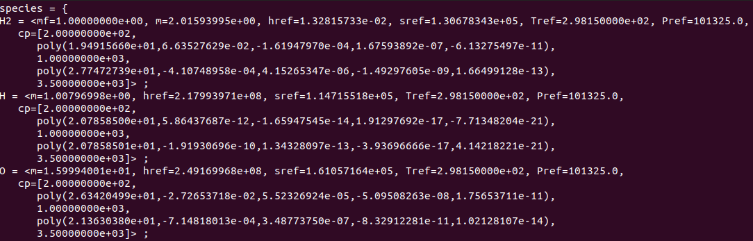
Sample .mdl file showing the layout of the data contained the file.

The Chemkin formatted thermodynamic database files look like the following:

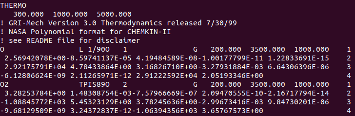
Sample of a .therm file showing the general structure of data within it.

The Chemkin formatted transport property database files have the following structure:

Sample of a .tran file showing the general structure of the data within it.

If you need a reaction section in the .mdl file, you need to pass a Cantera formatted YAML mechanism file to the script. If you have the chem.inp, tran.dat and therm.dat files already, you can generate a Cantera mechanism file via the following steps.

1. Install Cantera on your machine using: pip install cantera. This will install a version of the Cantera Python module on your machine. Additional tools are installed with this module, which you will now have access to.

2. Navigate to the directory containing the Chemkin files and run the following command: ck2yaml --input chem.inp --transport tran.dat --thermo therm.dat --permissive This will generate an output file called chem.yaml. This file will contain the species and reaction information that you will then provide to the chemkin-converter script to generate the .mdl file.

3. Call the chemkin-converter script with the --mechanism argument and pass it the name as follows: chemkin-converter --casename case --mechanism chem.yaml --chemkin

Creation of Model Files (.mdl) starting from Cantera YAML mechanism file

If you already have a Cantera formatted YAML mechanism file, you can generate a .mdl file that contains the species and reaction data with either of the following tools:

1. chemkin-converter --casename case --mechanism chem.yaml

2. cantera_to_mdl chem.yaml --casename case

Both commands generate:

• case.mdl

• case.tran

Use chemkin-converter when you need any of the following:

• species-name remapping (--species_name_remap)

• species subsetting (--species_subset and --species_subset_order)

• forcing no reactions (--remove_reactions)

• optional transport/ table generation (--transport_tables)

Use cantera_to_mdl when you only need a direct YAML conversion to Stream .mdl/.tran outputs.

Creation of Model Files (.mdl) from Species Lists and Existing Stream Artifacts

If you already have a Stream-format transport file and only need a selected species set, use the --species_only workflow. This is useful when creating smaller model files quickly without re-processing a full mechanism.

Required inputs:

• species_subset.txt (species names to retain)

• source .tran file (for example $CHEMISTRY_DATABASE/data_base/chemkin/air_5s17r.tran)

Optional input:

• source .mdl file (to preserve species definitions from an existing model file)

Command:

chemkin-converter --casename case --species_only --species_subset species_subset.txt --source_tran source.tran [--source_mdl source.mdl]

Output:

• case.tran subset to requested species

• case.mdl with matching species and empty reactions section

Creation of Model Files (.mdl) from RMG Species Inputs

For workflows that start from species structures (for example SMILES), Stream provides rmg_to_mdl. This utility queries RMG for thermo/transport data, emits Chemkin-form intermediates, and then calls chemkin-converter --chemkin to produce final artifacts.

Example:

rmg_to_mdl --casename case --species "H2" --species "O2" --species "N2"

Outputs:

• case.mdl

• case.tran

Additional options:

• --species_file: load species entries from file instead of repeated --species flags.

• --database_path: explicit path to RMG database root.

• --thermo_library: repeatable thermo-library preference list.

• --transport_library: repeatable transport-library preference list.

• --strict_transport: fail if any selected species lacks transport data.

• --transport_tables: also create a transport/ folder with *_vis.dat, *_con.dat, and *_dif.dat.

• --output_dir: directory for final artifacts.

• --keep_intermediate: keep generated Chemkin-format intermediate files.

Thermodynamic Models for Caloric Equation of State

The thermodynamic model for the caloric equation of state is selected using the run control file variable thermodynamic_model. One may choose any one of the following three specifications:

Example of a thermodynamic model specification

thermodynamic_model: vibrational
thermodynamic_model: curve_fit
thermodynamic_model: adaptive

If this variable is not present in the run control file, then the adaptive model is chosen by default. The adaptive model is not a model, but rather causes the code to use the curve_fit model if a \(C_{P}\) is specified or the vibrational model if a \(C_{P}\) is not specified.

The default caloric equation of state model is vibrational equilibrium model, which is the internal energy based on the assumption that the vibrational modes are in equilibrium. Assuming a harmonic oscillator for vibrational modes, the internal energy of the \(\text{i}^{\text{th}}\) species in the mixture is given by the following equation:

\[e_i(T) = \left( h_f \right)_i + R_i \biggl[ n_i T + \frac{\theta_{v,i}}{\theta_{v,i} \left( e^{\frac{\theta_{v,i}}{T}} - 1 \right)} \biggr]\]

The variables \(n_{i}\) and \(\theta_{v,i}\) are obtained from the species specification variables n and theta_v respectively. The variable \(\left( h_{f} \right)_{i}\) which represents the heat of formation, is computed from the species specification variables href and Tref.

The caloric equation of state can also be specified by providing curve-fit functions for \(C_{P}\). The curve-fit is specified over temperature intervals using a list of temperatures with curve-fit functions specified between the temperature intervals. Commonly used forms include poly and shomate (additional parser-accepted forms are listed in MDL File Syntax and Format Reference). The first is a fourth-degree polynomial given by the expression poly(A,B,C,D,E) where,

\[C_p = A + BT + CT^2 + DT^3 + ET^4\]

And the units are \(\frac{J}{mol \cdot K}\) . The following example shows the usage of this form in the definition of a \(C_{P}\) curve fit over three temperature intervals for hydrogen:

Polynomial curve-fit specification

H2: <cp=[75.0, poly(40.4475, -3.01156e-1, 2.35251e-3, -7.42018e-6, 8.35504e-9),
         300.0, poly(24.4709, 0.0289467, -6.46136e-05, 6.23552e-08, -2.09548e-11),
         1000.0, poly(25.4069, 0.004967, -1.39243e-08, -1.76658e-10, 2.09483e-14),
         5000.0]> ;

The second functional form, the Shomate form, is given by the expression shomate(A,B,C,D,E) where,

\[C_p = A + Bt + Ct^2 + Dt^3 + Et^{-2}\]

and where \(T(K)/1000\) and \(C_{P}\) is in units of \(\frac{J}{mol \cdot K}\). The following example shows the usage of this form in the definition of a \(C_{P}\) curve fit for \(H_{2}O\) from the NIST (National Institute of Standards and Technology) database, over two temperature intervals, one from 500-1700 Kelvin and another from 1700-6000 Kelvin.

Shomate curve-fit specification

H2O: <cp=[500.0, shomate(30.09200,6.832514,6.793435,-2.534480,0.082139),
         1700.0, shomate(41.96426,8.622053,-1.499781,0.098119,-11.15764),
         6000.0]> ;

Additional cp formats from the CHEM guide are NASA-7 and NASA-9:

\[\frac{C_p(T)}{R} = a_1 + a_2T + a_3T^2 + a_4T^3 + a_5T^4\]

\[\frac{C_p(T)}{R} = a_1T^{-2} + a_2T^{-1} + a_3 + a_4T + a_5T^2 + a_6T^3 + a_7T^4\]

These are specified as nasa7(...) and nasa9(...) in the same interval-list syntax as above (with nasa9r(...) and nasa9mks(...) also accepted by the parser). A compact example is:

NASA-9 curve-fit specification

O : <cp=[200.0,
         nasa9(-7953.6113,160.7177787,1.966226438,0.00101367031,-1.110415423e-06,6.5175075e-10,-1.584779251e-13),
         1000.0,
         nasa9(261902.0262,-729.872203,3.31717727,-0.000428133436,1.036104594e-07,-9.43830433e-12,2.725038297e-16),
         6000.0]> ;

For all \(C_P\)-based forms, provide consistent reference quantities (href, sref, Tref, Pref). In adaptive workflows, providing cp entries causes the curve-fit thermodynamic path to be selected.