Introduction

The Loci-Stream code is a product of the coupling of a CFD flow solver (Stream) to an open-source parallel-computing framework (Loci). Together the two components make up the Loci-Stream code. The Loci framework is a highly scalable framework that powers the Stream solver to run on large-scale machines with thousands of processors. Loci-Stream is designed to take advantage of existing commercially available front-end technology (standard grid generators) and back-end technology (post-processing software such as Tecplot, FieldView, EnSight etc.) which is relatively inexpensive compared to proprietary pre-processing and post-processing software provided by the major CFD vendors. The diagram below illustrates how typical users interact with Loci-Stream during a simulation workflow.

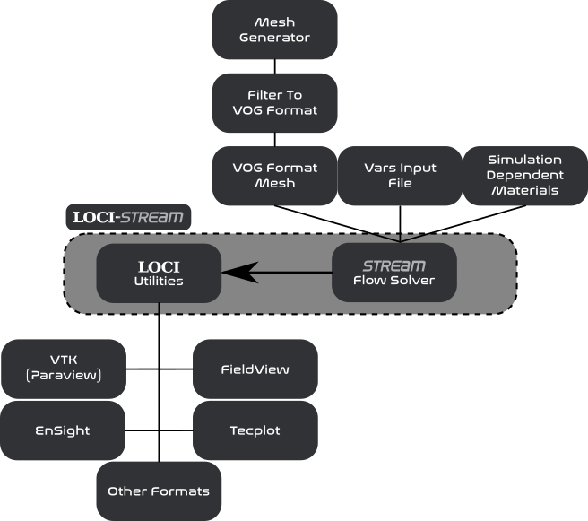
The organization of the Loci-Stream code.

Loci-Stream is a pressure-based finite-volume solver that operates with generalized unstructured meshes. Some of the major simulation capabilities include the following:

• Incompressible flows

• Compressible flows with shock, rarefaction, and expansion waves

• Turbulent flows using RANS, DES, and LES turbulence closure methods

• Cavitating flows using REFPROP tabulated fluids

• Combusting flows using finite-rate chemistry and flamelet-based tabulation methods

• Volume-of-fluid (VOF) simulations with multiple liquid materials

• Lagrangian particle simulations

• Generalized moving mesh simulations with overset grids

There are two files that are required for running a simulation: a grid file (.vog extension) and a run control file (.vars extension). The grid and control files are keyed to the case name which is supplied to the execution command. The following sections provide some basic information about these data files.

The general philosophy of this user manual is to teach by example with a set of examples that are sequentially more complex. Each new example introducing another layer of functionality in Stream. As such the earlier portions of the manual will contain the most detail and discussion of the details of using Stream, with subsequent sections relying on the user having read through the previous sections and building on that knowledge base.

Run Control File

The run control file contains all the input variables required to specify a simulation. The run control file sample in this section illustrates a lid-driven cavity simulation, where flow in a 2-D cavity is driven by a sliding lid. All variables in the run control file must be located within a single pair of squiggly brackets {}. Other than this constraint, there are no constraints on the location or order of the variables in the file. Generally, however, it is useful to keep the variables arranged in some logical groupings as shown in the run control file example so that information can be easily located. Detailed explanation of the input variables in each of the groupings can be found in later sections of this guide. Note that in general, one can include comments throughout the run control file using the // characters. All file contents located between the // and the end of the line will be ignored by the file parser.

The run control file variables that are required for a simulation are governed by the hierarchy of options that are selected. Some options will require a particular set of variables to specified, whereas other options may have different variables that need to be specified. This hierarchy includes elements such as the compressibility of the simulation, the presence of combustion or cavitation, the numerical methods selected to solve the governing equations, the forms of the governing equations, and the models used in the governing equations.

Sample run control file for lid-driven cavity flow

// Cavity flow, Re=1000.
{
// Grid file information.
grid_file_info: <file_type=VOG,Lref=1 m>

// Boundary condition information.
boundary_conditions:
<
BC_1=noslip, BC_2=noslip, BC_3=noslip, // left, right, bottom walls
BC_4=incompressibleInlet(v=-1.0 m/s), // lid
BC_5=symmetry,BC_6=symmetry // symmetry boundaries
>

// Initial condition.
initialCondition: <rho=1.0 kg/m/m/m,v=0.0,p=0.0>

// Thermodynamic and transport properties.
chemistry_model: air_1s0r
transport_model: const_viscosity
mu: 0.001

// Flow properties.
flowRegime: laminar
flowCompressibility: incompressible

// Time integration.
timeIntegrator: BDF
timeStep: 1.0e+30
numTimeSteps: 1001
convergenceTolerance: 1.0e-30
maxIterationsPerTimeStep: 1

// Fluxes and gradient limiting.
inviscidFlux: SOU
limiter: none

// Equation options.
momentumEquationOptions: <linearSolver=SGS,relaxationFactor=0.7, maxIterations=5>

pressureCorrectionEquationOptions: <linearSolver=PETSC, relaxationFactor=0.1, maxIterations=20>

// Output.
print_freq: 100
plot_freq: 100
restart_freq: 1000
}

Grid File

The only grid file format currently fully supported by Stream is the volume grid format (.vog extension). The only means of obtaining a grid in this format is to use the translators provided in the Loci distribution. These can be found in the /bin directory within the Loci installation directory.

Translators for generation of .vog files

Grid Format	Translation Procedure
CFD++	cfd++2xdr → xdr2vog
Cobalt Solutions	cobalt2vog
Fluent	fluent2vog
Plot-3D	plot3d2vog
SolidMesh/AFLR3	ugrid2vog

The table above shows some of the existing translators that are available, and the command used to produce a .vog file from the input grid file. As an example, if the AFLR3 mesh generator was used to generate a volume mesh, one would have a file called either case_name.ugrid or case_name.b8.ugrid, depending on whether the file was output in ASCII or binary form. To translate the file, one would issue the following command (assuming the grid was generated in units of inches):

ugrid2vog -in case_name

Following the completion of the translation, one should see the file case_name.vog in the directory where the command was issued. Note that while the grid may be generated in any units, upon translation, the internal units of the coordinates are in meters within the .vog file. All the translators shown in the table above require the units of the input grid so that coordinates can be scaled to meters for the output grid.

Execution Command

Below is an example command to run Stream within a Linux environment.

mpirun -np 10 stream –-scheduleoutput -q solution case_name >>&run.log &

A breakdown of the components of the command above is as follows:

• mpirun -np 10 stream: Execute stream in parallel using 10 processes. The number of processes to use in executing the computation is specified with the -np option. The number of processes that can be used depends on the size of the grid being used. On typical high-performance computing (HPC) systems, Stream exhibits excellent scalability down to about 5000 grid cells per process. Thus, for a grid of a million cells, one would typically use no more than 200 processes.

• –-scheduleoutput: The schedule file is a text-based file that contains the actual series of rules that are being executed by Stream. For single-process runs, this file is named .schedule, and will appear in the /debug directory if the --scheduleoutput argument is included on the command line. For multi-process runs, a series of files named .schedule-\* is generated, where the wildcard represents the process number(starting from 0). The schedule files are not typically of concern to the user during normal code usage, however, if a problem occurs, these files can be helpful to knowledgeable users in determining the cause of the problem.

• -q solution: The query value is passed to the code using the -q option on the command line. While other queries are possible with Stream, in practice, one will always pass the value solution, which indicates to the code that one wants the complete flow simulation solution.

• >>& run.log &: Stream writes out information to both standard-output and, should an error occur during code execution, to standard-error. This information can be redirected to a log file for permanent reference using the syntax >>& before the name of the log file on the command line. With this syntax, the file run.log will be created if it is not already present. If the file is already present, new information will be appended to the end of the existing run.log file. This is useful when conducting a restart so that the entire history of the run may be contained in a single file. If one uses the alternate syntax >&, any existing log file of the specified name will be deleted and a new log file created, thus destroying the information in the previous log file.