Simulation of Cavitating Flows

Stream can be used to simulate flows with cavitation by loading the cavitation module at run-time. This is done by inserting the following loadModule directive into the run control file as shown below.

loadModule: cavitation_nist
{
... standard run control file content
}

The cavitation_nist module uses tabulated REFPROP data for the equation of state and the fluid transport properties. The following sections discuss the analytical models for the cavitation source terms and provide information on the run control file variables required to perform simulations with the cavitation module.

Cavitation Model

Stream uses a homogeneous equilibrium model (HEM) to simulate the onset and evolution of cavitation within the fluid system. With such a model, the phases in the system (liquid, vapor, and non-condensable gas) are spatially averaged and assumed to occupy the same volume (homogeneously mixed). In addition, all phases are assumed to be in both mechanical and thermodynamic equilibrium, whereby the pressure, temperature, and velocity of the phases at any point are identical. The HEM is considered a good approximation for cavitating flows where the disturbance time scales and frequencies are long compared to the cavitation equilibration time. With these approximations, the continuity, momentum, and energy equations are solved for the mixture, rather than for the individual constituents of the flow. In addition, a transport equation for the vapor mass fraction is solved which contains source terms which generate vapor when the local flow pressure becomes lower than the vapor pressure of the fluid at the local temperature. A transport equation is also solved for the non-condensable gas (NCG) mass fraction. The transport equations for these two quantities are shown below:

\[\frac{\partial(\rho \alpha_v)}{\partial t} + \frac{\partial(\rho v_j \alpha_v)}{\partial x_j} = F(P, P_{\min}, F_{\max}, n) \cdot S(P, P_{vap}(T))\]

\[\frac{\partial \rho \alpha_{NCG}}{\partial t} + \frac{\partial \rho v_j \alpha_{NCG}}{\partial x_j} = 0\]

where \(\rho\) is the mixture density, \(v_j\) is the flow velocity, P is the static pressure, T is the temperature, \(\alpha_V\) is the vapor mass fraction, and \(\alpha_{NCG}\) is the non-condensable mass fraction . The following subsections describe the models that are available for the net vapor production rate source term \(S(P, P_{vap}(T))\) and the source term scaling factor \(F(P, P_{\min}, F_{\max}, n)\), which is can be activated in certain instances to prevent flow pressures from reaching unphysically low values.

Merkle Source Term Model

The Merkle source term model [MeFB1998] [HoAU2007] is a simple heuristic model in which the net vapor production rate is linearly proportional to the difference between the local flow pressure and the local vapor pressure. The expression for the net vapor production rate is given by the following:

\[S(P, P_{vap}(T)) = \rho(K_f \alpha_L + K_b \alpha_V)\]

where \(\rho\) is the mixture density, \(\alpha_L\) is the liquid mass fraction, and \(\alpha_V\) is the vapor mass fraction. The forward production and backward destruction rate coefficients \(K_f\) and \(K_b\) are given by:

\[\begin{split}K_f = \begin{cases} 0, & \text{if } P > P_{vap} \\ \frac{1}{\tau_{vap}}\left( \frac{P_{vap} - P}{\frac{1}{2} \rho_{\infty} U_{\infty} L_{\infty}} \right), & \text{if } P \leq P_{vap} \end{cases}\end{split}\]

\[\begin{split}K_b = \begin{cases} 0, & \text{if } P < P_{vap} \\ \frac{1}{\tau_{\text{cond}}}\left( \frac{P_{vap} - P}{\frac{1}{2} \rho_{\infty} U_{\infty} L_{\infty}} \right), & \text{if } P > P_{vap} \end{cases}\end{split}\]

In the expressions above, \(\tau_{vap}\) and \(\tau_{cond}\) are nondimensional source-term time-scale parameters associated with vaporization and condensation, respectively. The quantities \(\rho_{\infty}\), \(U_{\infty}\), and \(L_{\infty}\) are user-supplied reference density, velocity, and length values used to normalize the source term. In Stream, larger values of tauVap and tauCond make the Merkle source term weaker because \(K_f\) and \(K_b\) scale with \(1/\tau\). This convention differs from the coefficient-based form of the model often written in terms of multiplicative constants \(C_{vap}\) and \(C_{cond}\); when comparing against that form, the Stream inputs are related by \(\tau_{vap}=1/C_{vap}\) and \(\tau_{cond}=1/C_{cond}\). These parameters can be specified in the run control file using the names shown in the table below.

Merkle Source Term Model Tunable Parameters

Variable	Description	Typical Value
tauVap	Vaporization time-scale parameter	1
tauCond	Condensation time-scale parameter	80
L	Reference Length	None
V	Reference Velocity	None
rho	Reference density	None

The Merkle model can be selected by specifying source=Merkle in the cavitationEquationOptions variable as shown below.

cavitationEquationOptions: <linearSolver=SGS, relaxationFactor=0.9, maxIterations=5, source=Merkle>

The corresponding parameters for the model can then be set using the MerkleSourceParameters variable as follows.

MerkleSourceParameters: <tauVap=1.0, tauCond=80.0, L=0.7, V=1.5, rho=1.15>

Zwart Source Term Model

The functional form of the Zwart source term model [GeZB2004] is derived from the Rayleigh-Plesset equation which describes the growth or collapse of a vapor bubble in a pressurized fluid environment. Although more formally based on the physics of nucleation and vaporization, this model is none-the-less also ultimately heuristic in nature due to the introduction of constants that allow tuning of the vaporization and condensation rates for the problem of interest. The net vapor production rate is given by the following:

\[\begin{split}S(P, P_{vap}(T)) = \begin{cases} F_{vap} \frac{3 r_{nuc} (1 - \alpha_V) \rho_V}{R_B} \sqrt{\frac{2}{3}\frac{P_{vap} - P}{\rho_L}}, & \text{if } P \leq P_{vap} \\ F_{cond} \frac{3 \alpha_V \rho_V}{R_B} \sqrt{\frac{2}{3} \frac{P - P_{vap}}{\rho_L}}, & \text{if } P > P_{vap} \end{cases}\end{split}\]

where P is the local pressure, \(P_{vap}\) is the local vapor pressure, \(\alpha_V\) is the local vapor mass fraction, \(\rho_V\) is the local vapor density, \(\rho_L\) is liquid density, \(R_B\) is the bubble nucleation radius, and \(r_{nuc}\) is the nucleation volume fraction. The table below shows the default values for the user-tunable parameters for the model. Generally, unless specific knowledge is available regarding nucleation for a particular problem, one should only adjust the rate constants \(F_{vap}\) and \(F_{cond}\) to tune the model.

Zwart Source Term Model Tunable Parameters

Variable	Description	Default Value
FVap	Vaporization rate constant	50
FCond	Condensation rate constant	0.01
RB	Bubble nucleation radius	1.0e-06
aNuc	Nucleation volume fraction	5.0e-04

Sauer-Schnerr Source Term Model

The Sauer-Schnerr source term model [ScSS2008] is based on the Rayleigh-Plesset bubble dynamics equation. The expression for the net vapor production rate is given by the following:

\[\begin{split}S(P, P_{vap}(T)) = \begin{cases} F_{vap} \frac{\rho_v \rho_L}{\rho_m} \alpha_V (1 - \alpha_V) \frac{3}{R_B} \sqrt{\frac{2}{3}\frac{P - P_{vap}}{\rho_L}}, & \text{if } P < P_{vap} \\ -F_{\text{cond}} \frac{\rho_V \rho_L}{\rho_m} \alpha_V (1 - \alpha_V) \frac{3}{R_B} \sqrt{\frac{2}{3}\frac{P_{vap} - P}{\rho_L}}, & \text{if } P > P_{vap} \end{cases}\end{split}\]

Where \(\rho_L\) is the liquid density, \(\rho_V\) is the vapor density, \(\rho_m\) is the mixture density, \(\alpha_V\) is the vapor mass fraction, and \(R_B\) is the bubble radius. The bubble radius has the following definition.

\[R_B = \left( \frac{\alpha_V}{1 - \alpha_V} \frac{3}{4 \pi n} \right)^{\frac{1}{3}}\]

Where n is the bubble number density, and often takes a value around 1e+08. The table below describes the user tunable parameter for the model.

Sauer-Schnerr Source Term Model Tunable Parameters

Variable	Description	Default Value
rNuc	Nucleation radius	1.0e-5
n	Bubble number density	None

Source Term Scaling Factor

From the description of the source term models above, one can see that a specific functional relationship between the vapor production rate and the difference between the local flow pressure and the local vapor pressure is postulated. For the Merkle model a linear dependence is assumed while for the Zwart and Sauer-Schnerr models a square root dependence is assumed. For certain flow problems, the nature of the cavitation is such that neither functional dependence can provide an ample amount of vapor generation in certain regions without the pressure decreasing to values significantly below the vapor pressure and in certain cases becoming negative. This can result in the demise of the simulation. In practice, in any real device in which the flow is cavitating, the minimum pressure in the domain should remain in the vicinity of the local vapor pressure. In order that this can be achieved in numerical simulations without having to adjust the vaporization rate parameters to unrealistically high values (which would thus cause large amounts of vapor to be produced at all cells where \(P<P_{vap}\)), a source term scaling factor has been included in the formulation. This factor is only applied to locations in the domain where the pressure departs significantly from the local vapor pressure. The source term scaling factor \(F(P,P_{min},F_{max},n)\) is defined by the following expression:

\[\begin{split}F(P, P_{\min}, F_{\max}, n) = \begin{cases} F_{\max} + (1-F_{\max})\left[\frac{\exp\left(n\frac{P}{P_{\min}}\right)-1}{\exp(n)-1}\right], & \text{if } P \le P_{\min} \\ 1, & \text{if } P > P_{\min} \end{cases}\end{split}\]

The image below shows a plot of the function, while the table shows the default values for the scaling factor parameters. When \(F_{\max}>1\), the source term is amplified as pressure drops below \(P_{min}\). When \(0<F_{\max}<1\), the source term is damped as pressure drops below \(P_{min}\).

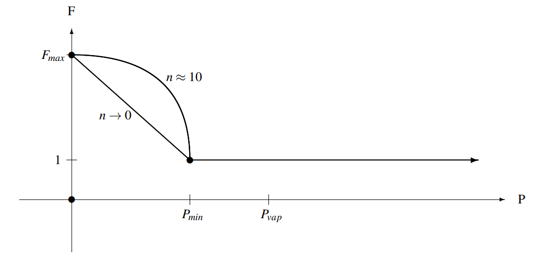
Source term scaling factor for controlling minimum simulation pressure. Scaling becomes active at user specified value of \(P_{min}\). User specified value \(F_{max}\) sets the low-pressure scaling factor, while user specified exponent \(n\) adjusts the scaling profile.

Source Term Scaling Parameters

Variable	Description	Default Value
cavitationMaxSourceFactor	Low-pressure scaling factor (\(F_{max}\))	1
cavitationSourceFactorExponent	Exponent	1
cavitationMinPressure	Scaling activation pressure	1

The value of \(F_{max}\) is usually problem dependent, however, the value in the table is a good starting point. The selection of \(P_{min}\) should be guided by actual experimental measurements on similar flow configurations if possible, however, if such information is not available, values in the range of no more than several hundred Pascals below the vapor pressure are recommended. In general, it is noted that the minimum simulation pressure will be somewhat below the specified value of \(P_{min}\) because this is merely the point at which the source term scaling is activated. The variables cavitationMinPressure and cavitationSourceFactorExponent should be non-zero to avoid division by zero in the scaling expression.

Control File Setup

Setting up a run control file for the simulation of a cavitating flow is like setting up a standard compressible flow problem. It is important to note that cavitating flows can only be simulated in compressible mode. A few important guidelines must be observed when setting up the run control file for a cavitation simulation:

• Boundary conditions must be set for the vapor mass fraction variable vapor_y and non-condensable gas mass fraction variable, NCG_y, on all inlet boundaries.

• Initial conditions must be set for vapor_y and NCG_y.

• The temperature form of the energy equation must be used by specifying form=temperature in the variable energyEquationOptions. The total enthalpy and total energy forms of the energy equation are not supported.

The specifications for vapor_y and NCG_y must always be provided. If there is no NCG in the flow, specify a value of 0. The following subsections detail each section of the run control file.

Boundary Conditions

Because cavitating flows must be simulated using compressible mode, the only inlet boundary conditions that should be in use are subsonicInlet, supersonicInlet, and inflow. The following shows an example of the specification of the vapor_y and NCG_y boundary condition for a subsonic inlet with pure liquid with a small amount of NCG:

Inlet=subsonicInlet(v=10.11 m/s, T=300.0 K, k=0.0, omega=1000.0, vapor_y=0.0, NCG_y=1.0e-06)

Similar specification would be made for the other inlet types.

Initial Conditions

The initial condition for the vapor and NCG mass fractions are set as follows:

initialCondition: <vapor_y=0, NCG_y=0.0, v=10.11 m/s, p=28515.8 Pa, T=300.0 K, k=0.0, omega=1000>

Similar specification of these values can be made using the run control file variables ql and qr or the variable initialConditionRegions as discussed in the following Appendix.

Equation of State and Transport Properties

The cavitation_nist module utilizes tabulated thermophysical property data from the NIST REFPROP software. A python utility is provided with the Stream source code that can generate tabulations for liquid, vapor, and saturation data files for any REFPROP species. The utility will generate three output files with suffixes of .liq, .vap, and .sat. The prefixes for the liquid and vapor files must be provided using the liquid_model and vapor_model variables in the run control file. The prefix for the saturation file will be taken from the liquid_model variable. The equation-of-state section in the run control file should look as follows:

liquid_model: NITROGEN
vapor_model: NITROGEN
transport_model: module

Setting the value of the transport_model to module indicates that all transport data is to be obtained from data in the tabulated liquid, vapor, and saturation files.

Some cavitation cases use temperature clip limits that place part of the requested vapor or liquid table on the opposite side of the saturation boundary. In those cases, the default REFPROP tabulator stops with an error because there is no stable pure-phase state to tabulate at those pressure levels. The cavitation REFPROP tabulator therefore provides an explicit --extend_to_phase_boundary option for users who still need a rectangular table for cavitation_nist. That mode writes a single saturation-boundary continuation row where needed, and only falls back to repeating the last continuation state if a later pressure level still requires continuation after the saturation curve has ended. This is a numerical compatibility option for the mixture model, not a way to create new exact pure-phase states. See REFPROP Tabulation Utility for details and usage guidance.

Cavitation Equation Options

An example of the cavitation equation section of the run control file with all available options is shown below:

cavitationEquationOptions: <linearSolver=SGS, relaxationFactor=0.9, maxIterations=5,
                            source=Zwart, vaporProductionRateRelaxationFactor=0.7>

ZwartSourceParameters: <RB=1.0e-06, aNuc=5.0e-04, fVap=50.0, fCond=0.01>
cavitationInviscidFlux: SOU
AlphaViscosity: 1.0e-05
liquid_rho: 736
vapor_rho: 17
NCG_rho: 15
cavitation: on
cavitationMinPressure: 3200
cavitationMaxSourceFactor: 100
cavitationSourceFactorExponent: 10
turbulentVapourPressureCorrection: on

The .vars file variables used are summarized in the table below.

Some Cavitation Module Options

Parameter	Description
AlphaViscosity	Artificial viscosity added to vapor and NCG mass fraction transport equations for numerical stability purposes.
cavitationInviscidFlux	Flux scheme used for vapor and NCG transport equations. Supported values are: FOU and SOU.
liquid_rho	Reference value for liquid-phase density used in normalizing the liquid term in the pressure-correction equation.
vapor_rho	Reference value for vapor-phase density used in normalizing the vapor term in the pressure-correction equation.
NCG_rho	Reference value for non-condensable-gas density used in normalizing the NCG term in the pressure-correction equation.
turbulentVapourPressureCorrection	Activates the turbulent correction to the vapor pressure.

The linear solver options are like the other governing equations that have been previously covered. All linear solvers discussed (here) are supported for the value of linearSolver, however one should rarely need to use anything other than the SGS solver. Source term model selection is made using either source=Merkle, source=SauerSchnerr, or source=Zwart. Common starting parameters for these three models are shown below:

MerkleSourceParameters: <tauVap=1.0, tauCond=80.0>
ZwartSourceParameters:<RB=1.0e-06, aNuc=5.0e-04, fVap=50.0, fCond=0.01>
SauerSchnerrSourceParameters: <rNuc=3.0e-06, n=4.8e8>

To explicitly turn off the source terms in the vapor mass fraction equation, one can specify cavitation: off in the run control file. The default value for this variable is on. Parameters for the source scaling model are specified using cavitationMinPressure, cavitationMaxSourceFactor, and cavitationSourceFactorExponent. If these are not specified, default values are used and the resulting scaling factor remains 1.0. If the liquid_rho, vapor_rho, and NCG_rho variables are not included (or are set to -1), the code will use local cell values to normalize the pressure-correction equation at each cell.

Non-Condensable Gas Specification

All cavitation simulations involve NCG terms in the governing equations, even if the user does not use NCG. The default fluid properties used for the nonCondensableGasProperties variable is air as shown below. To use a different fluid, the user must specify its molar mass m, specific heat at constant pressure cp, laminar dynamic viscosity mu, and thermal conductivity kcond in the nonCondensableGasProperties variable.

nonCondensableGasProperties: <m=28.9647 g/mol, cp=1005 J/kg/K, mu=1.805e-5 kg/m/s,
                              kcond=0.02476 W/m/K>

Output Variables

The table below shows additional field variables that are available for output in cavitating flow simulations. Default variables are output automatically and do not need to be specified in the plot_output line in the run control file.

Field Variable Output for Cavitating Flows.

Variable	Description	Default
bt`	Bulk expansion coefficient * temperature	No
F	Source term scaling factor	No
liquid_vof	Liquid volume fraction	No
liquid_y	Liquid mass fraction	No
NCG_vof	NCG volume fraction	No
NCG_y	NCG mass fraction	No
NCG_yResidual	NCG mass fraction eq. residual	No
pV`	Vapor pressure	No
rhoL	Liquid density	No
rhoV	Vapor density	No
vapor_y	Vapor mass fraction	No
vapor_vof	Vapor volume fraction	No
vapor_yResidual	Vapor mass fraction eq. residual	No

Practical Notes on Merkle Parameters

The Merkle model is often easiest to interpret in terms of back-of-the-envelope response times. For a local pressure departure \(\Delta P = |P_{vap}(T)-P|\), the Merkle source coefficients have the characteristic magnitude

\[K \sim \frac{1}{\tau}\left(\frac{\Delta P}{\frac{1}{2}\rho_{ref}V_{ref}^2}\right)\frac{V_{ref}}{L_{ref}}\]

which implies an effective local phase-change time scale of

\[t_{eff} \sim \frac{1}{K} \sim \tau\left(\frac{L_{ref}}{V_{ref}}\right) \left(\frac{\frac{1}{2}\rho_{ref}V_{ref}^2}{\Delta P}\right)\]

When \(\Delta P\) is of the same order as the reference dynamic pressure \(\frac{1}{2}\rho_{ref}V_{ref}^2\), this reduces to the useful estimate \(t_{eff} \sim \tau L_{ref}/V_{ref}\).

These estimates are only intended as order-of-magnitude guides, but they are useful when choosing starting values for tauVap and tauCond.

• tauVap and tauCond are heuristic closure parameters, not fluid properties.

• Smaller values of tau strengthen the source term and shorten the effective phase-change time scale. Larger values weaken the source term.

• Compare the estimated vaporization and condensation time scales against the residence time through the cavitating region and, when available, against experimentally observed cavity growth and collapse times.

• If the estimated vaporization time scale is orders of magnitude smaller than both the local flow time scale and the numerical time step, the source term may become extremely stiff and can drive pressures far below the local vapor pressure before transport balances the source.

• Because the normalization uses the supplied L, V, and rho values, raw tau values should not be compared across cases unless the reference values are also compared.

• For cryogenic flows, use the local temperature-dependent vapor pressure and any available pressure-depression or cavity-length measurements to guide the choice of a reasonable starting range.

REFPROP Tabulation Utility

The Python REFPROP tabulation utility is located under in the bin/ directory in the source code. The name of the utility is cav_tab_tool. This tool is for building necessary liquid, vapor, and saturation input files.

The Python tabulation utility has a functionality for making calls directly to REFPROP 11. This allows for the tool to tabulate as many pressure levels as the user desires. The user specifies the REFPROP material name, the pressure range, temperature range, and the number of data points to use over each range. The user can also pass a flag (--log_p) to uniformly distribute the pressure points in the log-space to ensure that an equal number of points resolve each pressure decade (this is good for large pressure ranges). The tool also supports adaptive temperature spacing (--adaptive_t) that places more points where the data is highly curved and fewer points where the data is nearly linear.

A set of .liq, .vap, and .sat files are generated by the tool, and these are the inputs used by the cavitation_nist module in Stream. Sample calls to the utility for the liquid/vapor files and the saturation files are given below.

There are two modes that the tool can be used in. One is for tabulating properties outside of a two-phase region in the thermodynamic space. The other is for tabulating the saturation curve properties of the liquid and vapor states.

Liquid/Vapor Tabulation

To generate tabulated liquid and vapor files, one should pass the liquidVapor argument to the tabulation tool. The presence of this argument enables a required set of arguments which are described below:

Liquid/Vapor Tabulation Arguments

Argument	Description
t_min	The minimum temperature range value
t_max	The maximum temperature range value
num_t	The number of temperature levels
p_min	The minimum pressure range value
p_max	The maximum pressure range value
num_p	The number of pressure levels
log_p	An optional argument that distributes the pressure levels uniformly across the logarithmic space of the pressure range
adaptive_t	Optional flag to enable adaptive temperature spacing
extend_to_phase_boundary	Optional flag to write a single phase-boundary continuation row when the requested temperature range contains no stable pure-phase state at a pressure level
t_rel_err	Relative error scale for adaptive spacing
t_abs_err	Absolute error scale for adaptive spacing
t_integrated_err	Target normalized integrated error used to stop adaptive refinement
t_min_points	Minimum number of temperature points used by adaptive spacing
t_max_points	Maximum number of temperature points used by adaptive spacing

If the log_p argument is not provided, a linear tabulation in the pressure dimension is performed. The logarithmic spacing enabled by the log_p argument creates a uniform spacing in the logarithmic space. This type of spacing is useful when there is a large variation in the pressure range, as a linear tabulation would result in a low resolution in the low-pressure region of the tabulation. An example command to generate liquid and vapor tabulation files for nitrogen in the temperature range of 65K-300K and pressure range of 50kPa-70MPa is shown below.

<StreamInstallDir>/bin/cav_tab_tool liquidVapor --fluid_name NITROGEN --t_min 65 --t_max 300 --p_min 50000 --p_max 70e6 --log_p --num_p 200 --num_t 200

In the example above, the liquidVapor argument sets the tool into the mode for tabulating .liq and .vap tables. The fluid_name argument must match an available REFPROP FLD file in the REFPROP fluid database. The tabulation levels are done at constant pressure, and so the t_min and t_max arguments are the temperature range over which to tabulate properties. The p_min and p_max arguments are the inclusive bounds of the pressure range over which you want to tabulate data. The log_p argument converts the pressure range into a logarithmic range and distributes points equally in that space and then converts back to pressure levels. This ensures an equal number of pressure levels per decade of pressure. This is sometimes a desirable option. The num_p and num_t arguments are the number of pressure levels to tabulate and the number of temperature levels to tabulate.

For some cryogenic cavitation problems, the requested (P,T) rectangle can cross onto the wrong side of the saturation boundary. A common example is a vapor table with T clipped low enough that no stable pure-vapor state exists above some pressure. In that situation the default behavior is to stop with an error because the requested phase does not exist in the specified temperature range.

If a rectangular table is still needed for cavitation_nist mixture-property lookups, the optional flag --extend_to_phase_boundary can be used. When enabled, the tool writes a single continuation row at pressure levels where the requested phase has no valid temperature window:

• For subcritical pressures, the continuation row is taken from the saturation boundary for that phase.

• If a later pressure level still needs continuation after the saturation boundary has terminated at the critical point, the tool reuses the last available continuation row as a fallback.

This option is intended for solver compatibility rather than for creating new thermodynamically exact pure-phase states. It should therefore be used deliberately and documented in the case setup.

An example command for a hydrogen vapor table that needs this continuation behavior is shown below.

<StreamInstallDir>/bin/cav_tab_tool liquidVapor --fluid_name HYDROGEN --t_min 16 --t_max 24 --p_min 20000 --p_max 6.0e6 --log_p --num_p 180 --num_t 160 --adaptive_t --t_rel_err 5e-4 --t_integrated_err 2e-3 --t_min_points 16 --t_max_points 450 --extend_to_phase_boundary

Saturation Tabulation

To generate a tabulated saturation file, one should pass the saturation argument to the tabulation tool. The presence of this argument enables a required set of arguments which are described below:

Saturation Tabulation Arguments

Argument	Description
t_min	The minimum temperature range value
t_max	The maximum temperature range value
num_t	The number of temperature levels
adaptive_t	Optional flag to enable adaptive temperature spacing
t_rel_err	Relative error scale for adaptive spacing
t_abs_err	Absolute error scale for adaptive spacing
t_integrated_err | Target normalized integrated error used to stop adaptive refinement
t_min_points	Minimum number of temperature points used by adaptive spacing
t_max_points	Maximum number of temperature points used by adaptive spacing

An example command to generate a saturation tabulation file for nitrogen in the temperature range of 65K-300K with 150 tabulation points is shown below.

<StreamInstallDir>/bin/cav_tab_tool saturation --fluid_name NITROGEN --t_min 65 --t_max 300 --num_t 150

In the example above, the saturation argument activates the saturation curve tabulation mode of the script. This mode has fewer arguments than the liquidVapor mode. The temperature range and number of points to include are the only arguments that are necessary. These arguments have the same meanings as they do for the liquidVapor mode of the tabulation tool that was discussed earlier.

Adaptive Temperature Spacing

When --adaptive_t is enabled, the tool refines the temperature grid by repeatedly splitting intervals that contribute the most interpolation error. The interpolation model remains piecewise linear; only the placement of points changes.

The adaptive controls have the following meanings:

t_rel_err

Relative error scale. A larger value is more permissive and usually produces fewer points.

t_abs_err

Absolute error scale. This is useful when a property crosses zero or is very small in magnitude.

t_integrated_err

Dimensionless global error target used to stop refinement. Smaller values add more points; larger values reduce points.

t_min_points

Minimum number of temperature points (safety floor).

t_max_points

Maximum number of temperature points (hard cap).

The integrated error used by the tool is a normalized quantity:

1. On each interval, evaluate the true property value at the midpoint.

2. Compare that midpoint value against linear interpolation from interval endpoints.

3. Normalize the midpoint error by t_abs_err + t_rel_err*scale, where scale is based on local property magnitude.

4. Use the largest normalized error across tabulated outputs for that interval.

5. Weight by interval length and sum over the full temperature range.

This produces a single dimensionless metric (the “integrated error”) that reflects both local interpolation quality and how much of the range is affected.

Practical tuning guidance:

• Start with --t_rel_err 0.02 --t_integrated_err 0.05 --t_min_points 6 --t_max_points 250.

• If files are too large, increase t_rel_err and/or t_integrated_err, or lower t_max_points.

• If interpolation quality is insufficient, decrease t_rel_err and/or t_integrated_err, or raise t_max_points.

• If t_max_points is reached, the tool reports a warning and stops refinement at the cap.

For current cavitation_nist code, saturation interpolation supports non-uniform temperature spacing, so adaptive spacing can be used for .sat files as well as .liq/.vap.

Using Cavitation Tabulation Tool

One must have version 11 of the REFPROP software to use the cavitation tabulation tool. A short tutorial on how to install the dependencies for the cavitation tabulation tool is presented below.

1. Download the REFPROP 11 software using the NIST downloader. This must be done on a Windows machine. The software will be downloaded into a directory named REFPROP.

2. Copy the REFPROP directory over to a Linux machine. The software can be put in a directory such as /home/<User>/software/refprop, where <User> would be your username on the machine). Note: do not rename the REFPROP source code directory because that may cause issues. For example, the path should look as follows: /home/<User>/software/refprop/REFPROP

3. Compile a local version of REFPROP on your Linux machine

   1. Do a recursive clone of the following repository: git clone --recursive https://github.com/usnistgov/REFPROP-cmake.git

   2. Go to the root of the cloned repository: cd REFPROP-cmake

   3. Create a build directory: mkdir build

   4. Change to the build directory: cd build

   5. Run cmake to configure the build: cmake .. -DCMAKE_BUILD_TYPE=Release -DREFPROP_FORTRAN_PATH=/home/<User>/software/refprop/REFPROP/FORTRAN

   6. Build the project: cmake --build .

4. Once the build is complete, a librefprop.so file should be found in the build directory. This shared library contains all the REFPROP functions that the Python wrapper will call. Move this file to the REFPROP directory created in step 2.

   1. Move the shared library file: mv librefprop.so /home/<User>/software/refprop/REFPROP

5. Set the environment variable RPPREFIX to point to the REFPROP directory that contains the shared library file.

   1. Add the following line to your .bashrc file: export RPPREFIX=/home/<User>/software/refprop/REFPROP.

   2. Make sure to source your .bashrc file after adding this line: source ~/.bashrc.

6. Clone the REFPROP wrappers directory into the /home/<User>/software/refprop directory using the following command: git clone https://github.com/usnistgov/REFPROP-wrappers

7. Create a Python3 environment with the REFPROP interface installed. This will provide a portable and dependable Python environment for running the tabulation tool. Go to your refprop directory and follow the steps below:

   1. Create a virtual environment: python3 -m venv refprop-env

   2. Activate the environment: source refprop-env/bin/activate

   3. Install numpy: pip install numpy

   4. Navigate to the REFPROP wrappers directory: cd /home/<User>/software/refprop/REFPROP-wrappers/wrappers/python/ctypes

   5. Install the python wrapper into the environment: python setup.py install

   6. To leave the virtual environment type: deactivate

One you are in the python environment, you can run the tabulation script and it should execute using calls to the REFPROP library.

References

[MeFB1998]

3. 12. Merkle, J. Z. Feng and P. E. O. Buelow, “Computational Modeling of the Dynamics of Sheet Cavitation,” in Proceedings of the 3rd International Symposium on Cavitation, Grenoble, France, 1998.

[HoAU2007]

1. Hosangadi, V. Ahuja and R. J. Ungewitter, “Analysis of Thermal Effects in Cavitating Liquid Hydrogen Inducers,” Journal of Propulsion and Power, vol. 23, no. 6, pp. 1225-1234, 2007.

[GeZB2004]

1. 7. Gerber, P. J. Zwart and T. Belamri, “A Two-Phase Flow Model for Predicting Cavitation Dynamics,” International Conference on Multiphase Flow, Yokohama, Japan, 2004.

[ScSS2008]

7. 8. Schnerr, I. H. Sezal and S. J. Schmidt, “Numerical investigation of three-dimensional cloud cavitation with special emphasis on collapse induced shock dynamics,” Physics of Fluids, vol. 20, 2008.