Simulation with Overset Grids

Stream can use overset grids for simulating cases that have complex geometries or require mesh movements. This capability is enabled by inserting the following loadModule directive into the run control file as shown below.

loadModule: overset
{
  ... standard run control file content
}

The following sections discuss the overset method used in Stream and provide information on the run control file variables required to perform simulations with the overset module.

Overset Method

Stream uses a standard overset method where a background mesh has component meshes overlayed on it, and appropriate hole-cutting and blanking of cells is performed. At the interfaces of the components, a buffer region of cells exists to provide an implicit interpolation between the overlapping meshes. Some definitions that are helpful when working with the overset module are:

Definitions of terms used in the overset method.

Term	Description
Blanked cells	Cells that have been assigned a flag that controls how the cells are to be used in the context of the overset method (the nomenclature for these markers is iblank=1, iblank=2, etc).
Hole cutting	The removal of irrelevant or unused cells from an overset computation
Component geometry	The rough geometric specification (provided in the control file) of a component mesh’s shape that is used to remove background mesh cells that “inside” the component mesh’s empty area.
Interface boundary	The outermost boundary of a mesh.
iblank=0 State	Cells where the governing equations are solved normally. Values are donated to interpolation.
iblank=1 State	Cells where the governing equations are solved normally. Values are not donated to interpolation.
iblank=2 State	Cells of this type are not computed (no equations are solved within those cells), they receive their values by interpolating from a cloud of points that comes from a set of cells with iblank=0 (which are from the background mesh).
iblank=3 State	Cells are not computed. Their current value is simply advanced with time.

The iblank=3 cells are often ones that lie outside the background mesh, or background cells that are deep within a component mesh beyond the interpolation layer. The iblank=1 state is not used often during the overset simulations and is included for possible future uses. The most relevant states are the iblank=0,2,3 states.

The overset method marks roughly three layers of cells inwards from the interface boundary on a component geometry’s mesh with the iblank=2 state. This means that the values in that buffer layer of cells on the component geometry’s mesh obtain their values from an interpolation from the cloud of points on the background mesh. For example, the pressure correction equation is solved on the iblank=0 cells of the component mesh, which are adjacent to the iblank=2 cells. When an iblank=0 cell requires information about its iblank=2 neighbor, a list of cells that are used to construct the neighbor’s value, and the corresponding interpolation weights from each of those cells is collected. These stencil weights are directly inserted into the matrix equation for the pressure correction equation to provide implicit coupling between a component mesh and the background mesh.

Overview of the method

What follows in this section is a more detailed review the overset framework. Start by examining the figure below. Here the gray cells are iblank=0, the green cells are iblank=2, and the red cells are iblank=3. The right element in the image is the component mesh, and a solid component boundary is shown on the far right side of the element. For this simple illustration the two grids overlap in a 1D manner. Note: The image shown is as if the two meshes were overlapping, but retaining the coloring scheme. They are shown separated in this figure first to help the reader understand the marking and coloring scheme.

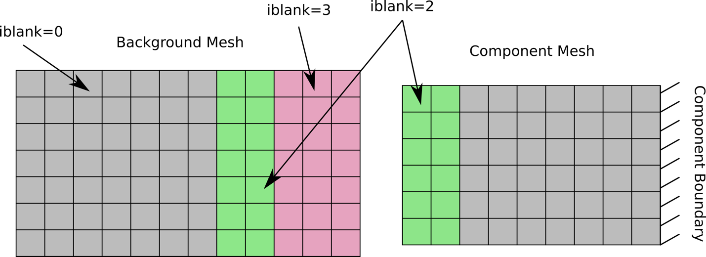
A background and component mesh that are separated. The coloring shows the iblank state as if they were on top of each other (as will be shown in later figures).

The figure below shows the two grids overlaid properly. The boundary of the component mesh has its outer layer marked as iblank=2, which draws from the iblank=0 background cells. The background mesh cells close to the component geometry’s solid surface are set to iblank=3, and a set of buffer layer cells on the background mesh around the iblank=3 cells are set to iblank=2, which they obtain their values from the iblank=0 cells on the component mesh.

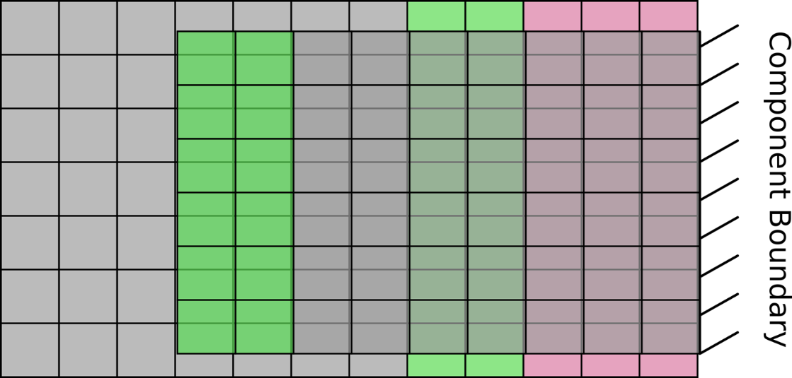
Both background and component meshes over each other. The iblank colors are consistent with the grid positioning.

The figure below shows an example case of how the implicit treatment is performed for the pressure correction equation. In this case, consider the cell A, which is located on the component mesh. It is gray, so it has a iblank=0 state, and the governing equations are solved on that cell. It requires information from its neighbor cells. The data about the cell to its right is easily obtained. The cell to its left (cell B) however is a green iblank=2 cell. So that cell’s data is coming from an interpolation that uses data from the gray background iblank=0 cells around it. The background cell centers are shown and numbered. The arrows point to the stencil of cells that hypothetically go into the interpolation for cell B. To construct the matrix equation for the pressure equation for cell A, one needs coefficient information from cells that contribute to the solution of cell A. This is how the equation \([A][P']=[b]\) is constructed. The difference here is that for cell A, the neighbor value of cell B is not used directly. Cell B’s data is a weighted sum of the values of the pressure correction of cell 1,2,3,4,5,6 in the diagram. These weights are directly inserted into the coefficient matrix for the pressure correction equation such that the equation for cell A contains entries from its right neighbor, and cells 1,2,3,4,5,6. This is then the equation that is solved.

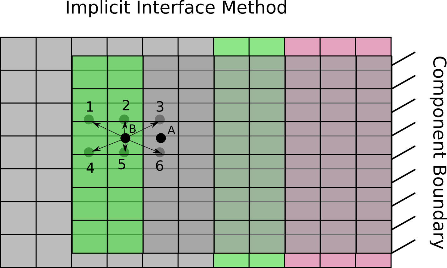
An example showing how the information for data from an iblank=2 cell is obtained from the cloud of points.

Pressure contours for a 2D plug/pipe case can be seen in the image below. Continuity of the solution across the overset mesh interface can be observed using the implicit method in this flow where a high pressure on left side of the domain flows over a plug and towards the right.

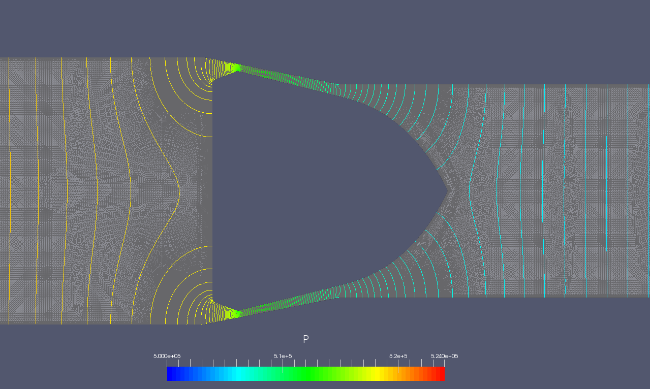
Pressure contours across the overset 2D sideways plug example case. Contours vary smoothly across the overset interface.

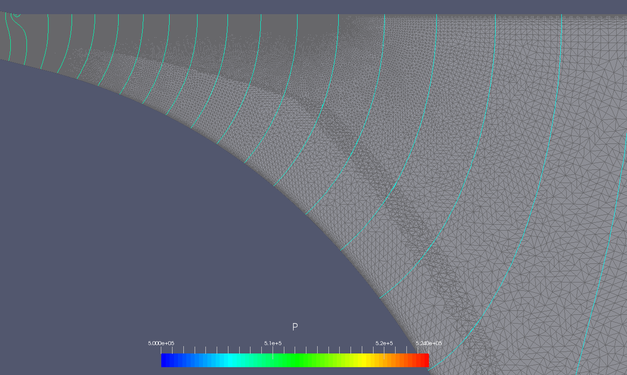
Pressure contours across the implicitly handled overset grid interface.

Control File Setup

Only a few additions need to be made to an existing run control file to set up an overset simulation. One thing to be aware of when setting up for an overset simulation is the specification of the componentGeometry variable as the overset algorithms depend on this variable being properly specified. The following subsections detail each section of the run control file.

Boundary Conditions

The boundary conditions for all the surfaces of both the background mesh and component meshes need to be specified in the boundary_conditions section of the run control file. The external mesh boundary of the component mesh needs to have an interface boundary specification as shown below for example.

overset_boundary=interface

In the above example the boundary name on the left of the = is whatever boundary name you have chosen for the mesh external boundary. No other adjustments need to be made to the boundary condition specifications section. Specify the other boundary conditions as you would for a non-overset simulation.

Initial Conditions

No changes to the initial conditions need to be made to accommodate an overset simulation.

Component Geometry

An important run control file specification that is required for overset simulations is the componentGeometry variable. This variable defines a region of the domain that should contain the inner volume of a component’s geometry. It does not have to be exact, but a close approximation will help the overset algorithm to properly mark and assign cells. The figure below shows an example diagram of an overset mesh configuration with the most common features named with the nomenclature used in this manual.

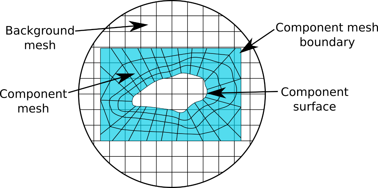
Diagram showing the important features of an overset simulation and the names used to refer to these features typically.

In keeping with the example shown above, the specification of a rectangular componentGeometry is shown the figure below. This rectangular region is what the overset algorithm uses to determine which background mesh cells should be marked with the non-participating iblank=3 state.

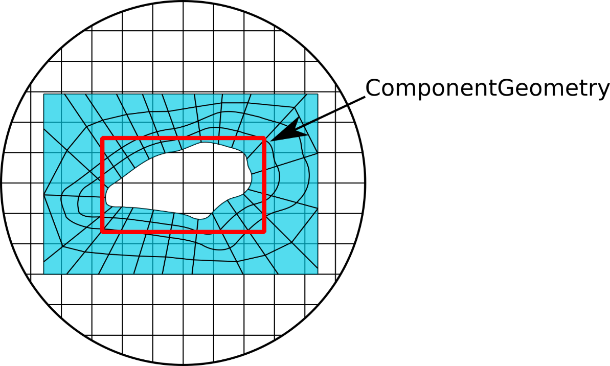
This is an example showing a rectangular componentGeometry specified to approximate the complex shape contained within it. The red rectangular region is what the overset algorithm uses to determine which background mesh cells to mark with the iblank=3 state.

An example of specifying the componentGeometry variable in the run control file is shown below.

componentGeometry: <body1=cylinder(p1=[-1, 0, 0], p2=[1, 0, 0], radius=3),
body2= sphere(center=[2, 2, 0], radius=1.5),
body3=revolution(p1=[5, 1, 1], p2=[7, 1, 1], radius=[2, 4, 3],
offsets=[0, 0.62, 1.0])>

Component geometries can be specified in terms of cylinders, spheres, bodies of revolution, or a list of planes. The table below contains examples of how to specify a component geometry of each type.

Types of primitives for defining a componentGeometry specification.

Variable	Description
cylinder(p1,p2,radius)	p1 and p2 define two end points of the cylinder axis and radius specifies the cylinder radius.
sphere(center,radius)	center and radius define the sphere’s center and radius.
revolution(p1,p2,radius,offsets)	Defines a body of revolution about an axis defined by points p1 and p2. radius specifies a list of radii along the axis between p1 and p2. offsets provides a list of the relative distance between p1 and p2 that the associated radii corresponds to.
planeList(list=[plane(p,n),…])	Defines a region that is on the left side of all the planes in the list. A plane is defined by a point, p, and a normal vector, n. The normal vector points out of the volume.

Examples of the component geometry forms described in the table above are show below.

A cylinder with an x-axis orientation from x=1 to x=2 with a radius of 0.5:

cylinder(p1=[1,0,0], p2=[2,0,0], radius=0.5)

A sphere centered at the origin with a radius of 1.5:

sphere(center=[0,0,0], radius=1.5)

A body of revolution with an x-axis orientation from x=1 to x=4.

revolution(p1=[1,0,0], p2=[4,0,0], radius=[3,2,4], offsets[0.0,0.6,1.0])

The body of revolution specification can be difficult to understand, so a diagram showing how each argument corresponds to a practical example is shown in below.

Body of revolution diagram showing the important quantities that must be specified in the componentGeometry entry.

A cube of edge length 1 centered at the origin:

planeList(list=[
   //x-coordinate planes
   plane(p=[1.0,0,0],n=[1,0,0]),plane(p=[-1.0,0,0],n=[-1,0,0]),
   // y-coordinate planes
   plane(p=[0,1.0,0],n=[0,1,0]),plane(p=[0,-1.0,0],n=[0,-1,0]),
   // z coordinate planes
   plane(p=[0,0,1.0],n=[0,0,1]),plane(p=[0,0,-1.0],n=[0,0,-1])
])

Component Motion

The overset module supports grid motions of the overset grids. This grid motion is not restricted solely to overset simulations, but this section is included here because often overset and grid motion are used together. The run control file entry for using moving grids is shown below for a case of a background and single component.

componentMotion:
<
  moving_part=prescribed,
  background_mesh=stationary
>

Three options are available to be assigned to each mesh tag in the run control file. The prescribed assignment means that the motion will be provided by an external input file. A rotation assignment can be given of the type rotation(axis=[1,0,0],center=[0,0,0],speed=400 rpm). The non-moving mesh should have the stationary assignment.

Any component mesh that is given the prescribed keyword in the run control file needs to have a corresponding file named motion_<meshTagName>.dat present at the same location at the run control

The elements of the motion file are described in the table below.

Field	Description
Number of interpolants	Number of interpolant inputs in the motion file
Time	Time in seconds
Position	Position in meters (3 components: x, y, z)
Quaternion	Four components of a normalized quaternion describing rotations about the preceding position

A cubic spline is used to interpolate between the given values. A discontinuity in the spline can be created if the condition for the same time is repeated twice.

A sample motion file is shown below. This one specified a translation in the x-direction of 63.5 mm in a span of 6 milliseconds. Note that the final digit of the quaternion should be 1.0 unless you are familiar with quaternions.

3
0.0 0.0 0.0 0.0 0.0 0.0 0.0 1.0
0.006 0.0 0.0635 0.0 0.0 0.0 0.0 1.0
10 0.0 0.0635 0.0 0.0 0.0 0.0 1.0

Output Variables

• The table below shows additional field variables that are available for output in overset flow simulations. Default variables are output automatically and do not need to be specified in the plot_output line in the run control file.

Field Variable Output for Overset Simulations

Variable	Description	Default
	No current outputs for overset module supported

Creating the Overset VOG Mesh with Tags

Overset meshes have multiple distinct meshes, but a single vog formatted mesh file is still required when using the overset module. This means that all the grids that compose the background and component meshes must be encoded into a single vog mesh file. Consider a case where a background mesh called backgroundMesh.vog and a component mesh called componentMesh.vog are to be used for an overset simulation. The following Loci utility is used to merge these two meshes into a single vog mesh named mergedMesh.vog with tags assigned to each mesh.

vogmerge -g backgroundMesh.vog -tag background -g componentMesh.vog-tag component -o mergedMesh.vog

The tags are important because they are what is used to reference the difference meshes when describing the different components in the run control file. The tag names are arbitrary.

Known Issue with Overset Module & Hole Cutting

While using the overset module you may notice a situation in your domain where there are gaps in the domain: cells missing like what is shown in the figure below. This is very often an effect of an interaction in the Loci framework between the componentGeometry specification provided in a run control file and the mesh of a component. The hole cutting (removal of cells) is done to save computational resources because there is no reason to simulate cells in the background mesh that would be wholly contained within body of a component mesh. The componentGeometry specification is what informs the overset algorithm about which cells are potentially within the body of a component mesh’s geometry, and it is this specification which often leads to situations like what is shown below.

A y-plane cute that is made through a domain to illustrate the hole cutting issue.

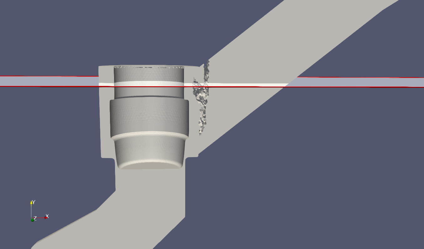
The region with the missing cells can be seen better in the image shown below, which is a top view of the plane cut shown above. In this figure, the component geometry was set to a large diameter (seen as the gap on the far-right side) for illustrative purposes. The gap seen on the left semicircular region is where the issue being discussed occurs.

Overset hole cutting leaving a gap over on the left between the plug and valve. The hole on the right was expected to be there due to the component geometry being set to that location.

The blanking of the cells close to the interface boundary of a component mesh reduces the amount of usable grid near the overlap region and this interacts with the Loci framework’s medial cut procedure which causes there to be insufficient overlap to fully connect the grid system. For this illustration, if the radius of the componentGeometry cylinder in this example is reduced from 0.056m to 0.047m, then there is sufficient overlap to prevent the gap. The user should err on the side of greater overlap between the component mesh’s interface boundary and componentGeometry specified surface. This can be done in this case either by slightly increasing the grid resolution in the overlap region to allow more cells to overlap, or by keeping the same resolution and pushing the componentGeometry further away from the interface as changing radius from 0.056m to 0.047m does in this example.

The left cut-plane shows the effect of setting the componentGeometry surface too close to the location of the boundary of the mesh for the component. On the right, the componentGeometry boundary definition was moved inwards, which allowed for more of an overlap region between the background mesh cells and the component mesh.

Another alternative approach to alleviate this issue is to simply extend the actual spatial extent of the component mesh to extend completely outside of the background mesh. This is more costly than the example above but may be an effective and fast solution for cases where adjusting the component geometry specification continues to cause issues with the gaps in the mesh.

Visualizing the iblank state of a simulation

A vars file option plot_overset_freq is available. This operates on the same principle as the plot_output vars file variable. If this variable is included, the output will be .csv files. There will be one file at each timestep output for each iblank state.

A helpful thing to keep in mind is that the iblank=3 cells are often ones outside of the domain, or within a component’s geometry. For the purposes of illustration, we will consider the case of a simple valve and plug configuration as shown below. The valve is the orange and is the background mesh, and the plug is the blue and is the component geometry.

2D valve overset domain. Blue is the plug, and orange is the fluid(background) domain.

Any overset simulation can be visualized using Paraview. Note: This visualization is for determining the state of the cells of the overset meshes in the event any debugging may be necessary. The standard extract utility works for overset simulations and presents the cumulative picture of the overset interpolating/hole cutting algorithm. The method for examining overset cell marker data in Paraview is:

1. Load the CSV file into Paraview (make sure to set the Field Delimiter Characters option to be a space)

2. Apply a Table to Points Filter to the loaded dataset.

3. Select the X Column, Y Column, and Z Column to be the x, y, z headers from the CSV file. If the file was read correctly in Step 1, the dropdown menu should show you x,y,z as data you can select for this part.

It is recommended to load both geometry files (fluid background mesh and plug component mesh) into Paraview along with the CSV data loaded using the process outlined above. Careful attention must be paid to which cells centers the red and green dots are aligned with. In the image below, if the red dots align with the cell centers of the left grid, then they are representing the iblank=3 state of the fluid mesh cells.

Side-by-side image of the iblank dataset (red and green dots) overlayed on the fluid(left side) and plug(right side) meshes.

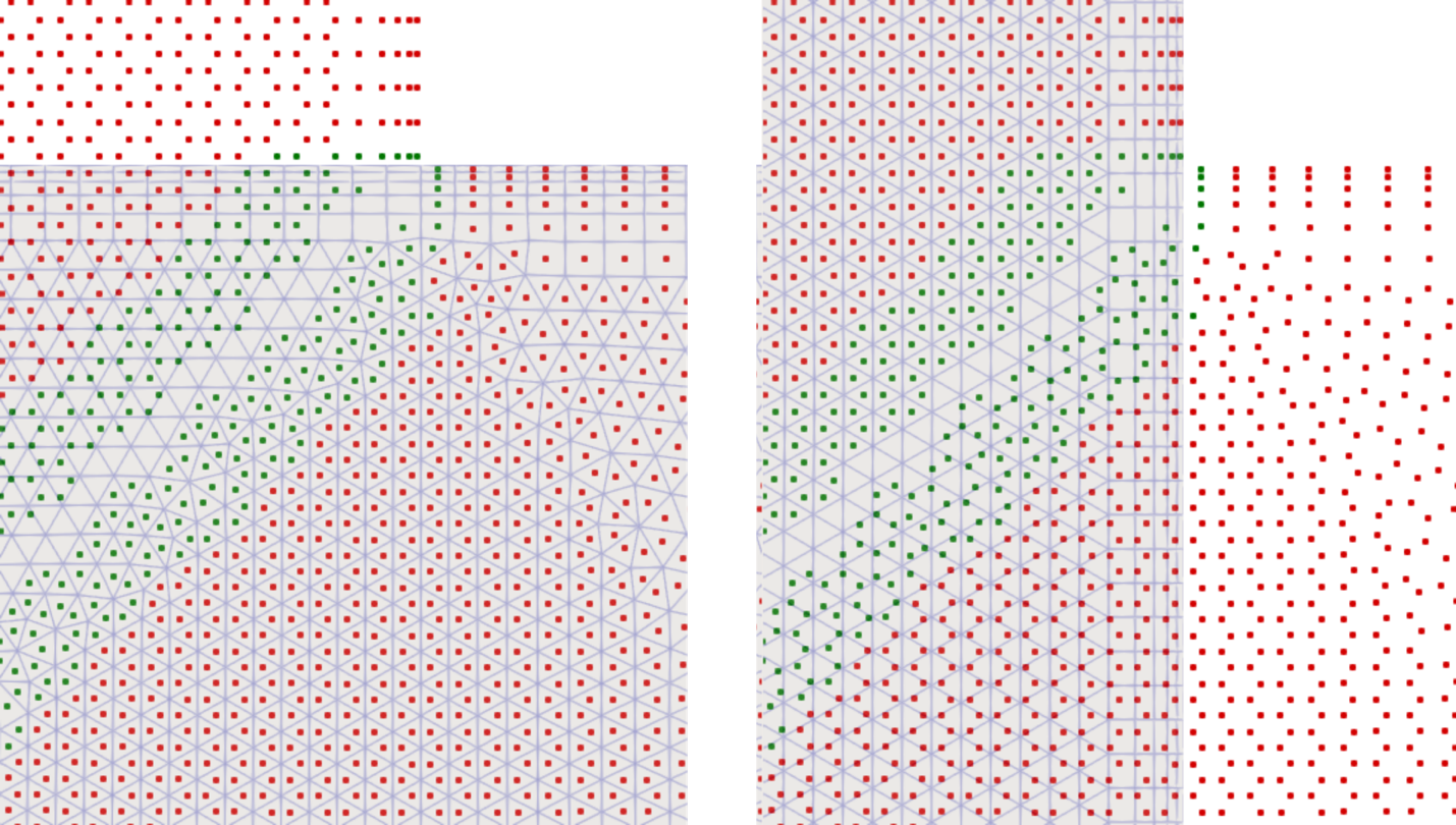
Left is the fluid mesh, and right is the plug mesh. Note the alignment of the red and green cells on the left and right meshes.

In the image aboe, the left image is the background fluid mesh, and the right images if the plug component geometry mesh. As was mentioned earlier, this image was created by loading the background fluid mesh, and the plug overset mesh separately into Paraview and displaying the iblank dataset over both grids. This is the region where the plug intersects the fluid mesh, on the left side of the plug. The vertical red/green lines that represent the background fluid mesh’s boundary layer are helpful for visually estimating where the plug is located on the background mesh. The background mesh cells that are within the plug’s no-slip surface boundary are marked with iblank=3. There is also a region around the plug akin to a buffer layer that is specified using the componentGeometry vars file specification which cuts out any of the background mesh that is contained within the boundaries of its specification. Ideally in this example, we only need an overlapping region of cells near where the outer boundary of the plug mesh’s grid is, so if the plug mesh has a much larger mesh compared to the geometry that is represented by the plug, the componentGeometry can be specified to remove additional cells.

Going back the left image, therefore the red markers don’t follow a simple straight line upwards. Because the compoenentGeometry is defined to be offset from the actual plug surface.

On the left image there are green markers that are aligned with the background mesh. These are iblank=2 cells. They are cells that are receiving their values from the iblank=0 cells that are used to make up the cloud of points for interpolation.