2. The Solution Algorithm

This chapter presents the pressure-based solution methodology used in Stream. It first motivates the all-speed pressure-based formulation, then gives a high-level map of the segregated nonlinear iteration, the notation used in the chapter, and the compact pressure-correction form that underlies the SIMPLE/SIMPLEC-family algorithms. The corresponding unstructured-grid discrete equations used in implementation are presented in Chapter 3.

The classical two-dimensional Cartesian derivation of SIMPLE and SIMPLEC is retained as background in the classical Cartesian pressure-correction appendix.

2.1. Pressure-Based Algorithms for All-Speed Flows

For incompressible flows, density has no role to play in the governing equations – it is either constant (for isothermal flows) or is a function of temperature (and not pressure). Thus, the continuity equation, which is typically used as a transport equation to compute density can no longer be used in its original form in the so-called density-based algorithms; the system of equations becomes stiff as the Mach number approaches zero. This can be addressed by employing special techniques such as preconditioning; however, in the low Mach number limit this can still cause some robustness and accuracy issues. Pressure-based algorithms, on the other hand, treat pressure as a solution variable and construct a transport equation for pressure by combining the continuity and momentum equations. Thus, there is no stiffness issue as the Mach number approaches zero. Moreover, pressure-based algorithms can be extended for compressible flows in a straightforward manner: simply tack on the energy equation and use the equation of state to obtain density from pressure. It must be emphasized that pressure-based algorithms still ultimately solve the original system of equations (the Navier-Stokes equations) without any compromise in accuracy across the Mach-number range, provided the appropriate flux discretization is used.

The stream flow solver therefore employs an all-speed pressure-based methodology. The mainline solver is built around the SIMPLE and SIMPLEC algorithms and the related SIMPLER family. Separate PISO-type and PIMPLE-type formulations are also available elsewhere in the code base. stream employs a spatially and temporally second-order accurate discretization methodology on generalized unstructured grids. It uses a finite volume method (FVM) with a collocated arrangement for the velocity components and the scalar variables like pressure and density. For incompressible flows, pressure-velocity decoupling is prevented by employing the so-called momentum interpolation approach; this involves adding a fourth-order pressure dissipation term while estimating the mass flux at the control volume interfaces.

For compressible flows, characteristic-based schemes (such as AUSM and SLAU) are employed. The velocity components are computed from the respective momentum equations. The velocity and the pressure fields are corrected using a pressure correction (\(p^{'}\)) equation. The correction procedure leads to a continuity-satisfying velocity field. The whole process is repeated until the desired convergence is reached. Relevant details of the implementation of stream are discussed in Chapter 3.

2.2. High-Level Solution Flow

The pressure-based algorithm is easiest to understand first as an information-flow picture. At the start of one nonlinear iteration, collect the current known state into

(2.2.1)\[Q^{it} = \left( \vec{u}^{\,it}, p^{it}, \dot{m}^{\,it}, \rho^{it}, \Phi^{it} \right),\]

where \(\Phi\) denotes the non-pressure scalar and thermochemical state. Depending on the model, \(\Phi\) may contain total energy, total enthalpy, temperature, species mass fractions, turbulence variables, volume-fraction variables, or other transported scalar fields. Within one nonlinear iteration, the scalar block produces an updated scalar state, \(\Phi^*\), from the current flow state. The momentum and pressure-correction branch uses the current iteration pressure, density, and closure data, including \(\Phi^{it}\) through the assembled coefficients and source terms, to update pressure, velocity, and face flux. The pieces meet again when the equation of state rebuilds density and the thermodynamic state.

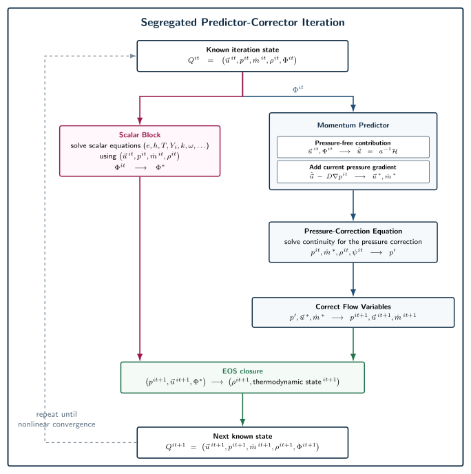
Fig. 2.2.1 High-level information flow for one pressure-based segregated predictor-corrector iteration in the compressible solve. The arrows show the mathematical data dependence, not a strict implementation schedule for every algorithm variant.

The figure is also the safest way to read the starred quantities in this chapter:

Symbol	How to read it in the algorithm picture
\(Q^{it}\)	The known state at the start of nonlinear iteration \(it\).
\(\Phi\)	The bundled scalar / thermochemical state, e.g. \(e\), \(h\), \(T\), \(Y_i\), and other transported scalars.
\(\Phi^*\)	The updated scalar state produced by the scalar equations during this nonlinear iteration.
\(\vec{u}^*\), \(\dot{m}^*\)	The momentum-predictor velocity and face flux before pressure correction.
\(p'\)	The pressure correction obtained from the pressure-correction equation built from continuity, provisional fluxes, and the EOS pressure response.
\(p^{it+1}\), \(\vec{u}^{\,it+1}\), \(\dot{m}^{\,it+1}\)	The pressure-corrected flow variables passed to the next nonlinear iteration.
\(\rho^{it+1}\)	The density obtained after EOS closure using the corrected pressure / velocity and the scalar-star state.

In pseudocode form, the same idea is:

given the converged state at time level n

for each new time level n+1:
  initialize Q^0

  for each nonlinear iteration it:
    solve scalar equations for Phi using the current flow state:
      (u^{it}, p^{it}, mdot^{it}, rho^{it}) -> Phi*

    build the pressure-free momentum predictor and include p^{it} using the current scalar / closure state:
      Phi^{it} -> u*, mdot*

    solve the pressure-correction equation from continuity, provisional fluxes, and the current EOS pressure response:
      u*, mdot* -> p'

    correct pressure, velocity, and face flux
      p' -> p^{it+1}, u^{it+1}, mdot^{it+1}

    apply EOS closure using corrected pressure / velocity and Phi*
       p^{it+1}, u^{it+1}, mdot^{it+1}, Phi* -> rho^{it+1} and thermodynamic state for the next iteration

  when the nonlinear iteration converges:
    final Q^{it} becomes the state at time level n+1

This picture is more important than the superscript convention. A star means “the intermediate quantity produced by the step that owns it.” Thus \(\vec{u}^*\) is a momentum-predictor velocity, while \(\Phi^*\) is a scalar-equation result. They are both intermediate quantities, but they do not mean the same stage of the algorithm.

The unstructured-grid pressure-correction forms in Chapter 3 show how this same branch is assembled in the actual finite-volume equations.

2.3. Notation Used In This Chapter

The symbols below are used throughout the pressure-based algorithm discussion.

Symbol	Meaning
\(n\)	Time level. A converged time step advances the solution from \(n\) to \(n+1\).
\(it\)	Nonlinear outer-iteration level inside the new time step.
\((\cdot)^*\)	Intermediate result produced by the equation block being discussed.
\((\cdot)'\)	Correction obtained from the pressure-correction equation.
\(\hat{\cdot}\)	Pressure-free contribution formed from the non-pressure part of the momentum equation.
\(P\), \(N\), \(f\)	Location labels: cell \(P\), neighboring cell \(N\), and face \(f\).
\(\left.\cdot\right\rvert_{(\cdots)}\)	Evaluation at the listed state.

A useful mental picture for one time step is

(2.3.1)\[(\cdot)^n \;\longrightarrow\; (\cdot)^{it} \;\longrightarrow\; (\cdot)^* \;\longrightarrow\; (\cdot)^{it+1}.\]

The star is local to the step that produces it. Thus \(\vec{u}^*\) is a momentum-predictor velocity, while \(\Phi^*\) is a scalar-equation result. They are both intermediate quantities, but they do not denote the same stage of the algorithm.

2.4. SIMPLE-Family Pressure-Correction Form

The relations below provide a compact solver-oriented summary of the pressure-based method. They are intended as the chapter’s main algebraic picture, while Chapter 3 gives the corresponding unstructured-grid discrete form used in stream.

Following standard SIMPLE/SIMPLEC nomenclature, the velocity and pressure corrections are introduced as:

(2.4.1)\[\begin{split}p &= p^* + p', \\ \vec{u} &= \vec{u}^* + \vec{u}'\end{split}\]

In the iteration-level notation used in Fig. 2.2.1, the pressure reference \(p^*\) is the pressure already available at the start of the nonlinear iteration, so \(p^* \equiv p^{it}\). The velocity \(\vec{u}^*\), by contrast, is the provisional velocity produced by the momentum predictor.

Assumptions In The SIMPLE-Family Correction

This section describes the shared pressure-correction form used by SIMPLE and SIMPLEC-like methods. The key assumptions are:

• The momentum equation is linearized at the current nonlinear iteration. Coefficients, source terms, density, transport properties, turbulence quantities, and other closure data are assembled from known or lagged states so that the momentum predictor is a linear solve for \(\vec{u}^*\).

• The pressure \(p^*\) is the current pressure reference used in that predictor, not a new converged pressure field.

• The hatted velocity \(\hat{\vec{u}}\) is the pressure-free part of the assembled linearized momentum row. It is not a separate pressureless physical solution.

• The pressure correction step treats the non-pressure thermodynamic / scalar state as fixed while estimating the pressure-induced density response.

• The velocity and face-flux corrections use an approximate momentum inverse. In SIMPLE, the neighbor velocity-correction terms are neglected in the correction relation. In SIMPLEC, those terms are approximated more consistently, which modifies the effective correction coefficient but leaves the same predictor-corrector sequence in place.

At a given nonlinear iteration, the momentum equations are solved using the currently available pressure field. The resulting provisional velocity is called the momentum predictor because it is the velocity predicted from the momentum equations before discrete continuity has been enforced. In cell \(P\), that predictor is written compactly as:

(2.4.2)\[a_P \vec{u}_P^* = \sum_{N\in\mathcal{N}(P)} A_{PN}\vec{u}_N^* + \vec{b}_P^* - \Omega_P \nabla p_P^*\]

Here \(\mathcal{N}(P)\) is the set of cells coupled to cell \(P\), \(A_{PN}\) are the neighbor coefficients, and \(\vec{b}_P^*\) contains the non-pressure terms that are already known when this predictor is assembled. It is convenient to collect those non-pressure terms into the shorthand

(2.4.3)\[\mathcal{H}_P(\vec{u}^*;\Phi_P^{\mathrm{lag}}) \equiv \sum_{N\in\mathcal{N}(P)} A_{PN}\vec{u}_N^* + \vec{b}_P^*,\]

so that the same momentum row becomes

(2.4.4)\[a_P \vec{u}_P^* = \mathcal{H}_P(\vec{u}^*;\Phi_P^{\mathrm{lag}}) - \Omega_P \nabla p_P^*\]

where \(a_P\) is the central coefficient of the component momentum equation (read componentwise in this vector shorthand), \(\Omega_P\) is the cell volume, and \(\Phi_P^{\mathrm{lag}}\) denotes the currently known thermodynamic / closure state in cell \(P\). That state may include quantities such as density, temperature, species composition, volume fraction, viscosity, turbulent viscosity, or other lagged model fields that affect the coefficients and source terms in the momentum row. These are not additional unknowns of the momentum solve; they enter only parametrically through the assembled coefficients and explicit terms. The symbol \(\mathcal{H}_P\) is an algebraic shorthand for “everything in the assembled momentum row except the diagonal term \(a_P\vec{u}_P^*\) and the cell-centered pressure-gradient term.” Depending on the formulation, \(\vec{b}_P^*\) may contain time-history terms, lagged nonlinear contributions, body-force/source terms, under-relaxation terms, and other explicit pieces.

Defining a hatted velocity,

(2.4.5)\[\hat{\vec{u}}_P = \frac{\mathcal{H}_P(\vec{u}^*;\Phi_P^{\mathrm{lag}})}{a_P}\]

We can write the momentum predictor provisional velocity as:

(2.4.6)\[\vec{u}_P^* = \hat{\vec{u}}_P - \frac{\Omega_P}{a_P}\nabla p_P^*\]

the meaning becomes clearer: \(\hat{\vec{u}}_P\) is the pressure-free predictor, namely the velocity obtained from the non-pressure part of the assembled momentum row. It is an intermediate algebraic quantity, not a separate physical state that satisfies continuity. The starred velocity \(\vec{u}_P^*\) is the corresponding provisional cell-centered velocity after the current pressure field \(p^*\) has been included in the momentum row. Note that the hatted velocity is the same quantity that later appears in the momentum-interpolation / Rhie-Chow face-velocity construction.

At this point, we have solved a linearized momentum equation to get a provisional velocity field \(\vec{u}^*\). This is the “momentum predictor” step. The next step is to check whether that provisional velocity satisfies the discrete continuity equation. If it does not, we need to compute a pressure correction \(p'\) that will modify the velocity and face fluxes so that the corrected solution satisfies continuity. For this stage, we consider the mass flux through each face, because the discrete continuity equation is enforced in terms of face fluxes: \(\dot{m}_f=\left[\rho(\vec{V}\cdot\vec{A})\right]_f\). In reality, it is simply the velocity that is actually being considered, but this mass flux quantity is easier to think about due to it being the thing that dictates the continuity equation’s solution. Let’s write the continuity in integral form over a faceted fixed control volume \(P\):

(2.4.7)\[\frac{d}{dt}\int_{\Omega_P}\rho\,d\Omega + \oint_{\partial\Omega_P}\rho\,\vec{u}\cdot\hat{\vec{n}}\,dA = 0\]

Approximating the volume integral by the cell-average density, \(\int_{\Omega_P}\rho\,d\Omega \approx \Omega_P \rho_P\), and the surface integral by a sum over faces gives, for a fixed control volume,

(2.4.8)\[\Omega_P\frac{d\rho_P}{dt} + \sum_{f\in\partial P}\left[\rho(\vec{u}\cdot\vec{A})\right]_f = 0\]

The mass face flux is defined as:

(2.4.9)\[\dot{m}_f=\left[\rho(\vec{u}\cdot\vec{A})\right]_f\]

With that, our continuity equation for cell P can be written as:

(2.4.10)\[\Omega_P\frac{d\rho_P}{dt} + \sum_{f\in\partial P}\dot{m}_f = 0\]

The continuity equation does not ask directly whether the cell-centered velocity \(\vec{u}_P^*\) is “correct.” What it asks is whether the net mass crossing the faces of cell \(P\) is balanced. A cell-centered velocity by itself does not answer that question, because mass conservation depends on the velocity component normal to each face, multiplied by face area and density. That is why the provisional momentum solution must be converted into provisional face fluxes before continuity can be checked. This is also why the pressure-correction equation is naturally written as a correction to face fluxes rather than as a direct replacement for the momentum solve. The momentum equation gives a provisional cell-centered velocity field. From that field we construct provisional face mass fluxes \(\dot{m}_f^*\). Continuity is then evaluated on those face fluxes. If the resulting cellwise mass balance is not zero, the pressure-correction step computes the change in pressure needed to modify the face fluxes so that the corrected fluxes satisfy continuity. For a focused discussion of why this remains meaningful in compressible flow, where density can change, see How Does Continuity Know The Provisional Velocity Is Incorrect?.

The provisional momentum predictor must be converted into a provisional face mass flux. On a collocated grid, that face flux is not obtained by a plain interpolation of cell-centered velocities alone; it also includes the usual momentum-interpolation (Rhie-Chow-type) pressure-coupling term. The provisional face mass flux associated with the momentum predictor is therefore written in compact form as:

(2.4.11)\[\dot{m}_f^* = \rho_f \hat{\vec{u}}_f \cdot \vec{A}_f - d_f \left( p_1^* - p_0^* \right) + \dot{m}_{f,\rho}^*\]

The first term is obtained from the face-interpolated hatted velocity and represents the transported pressure-free part of the flux. The second term restores the pressure coupling at the face, which is exactly what is needed to suppress collocated-grid checkerboarding. The remaining term, \(\dot{m}_{f,\rho}^*\), denotes the compressible density-correction contribution, which vanishes in the incompressible limit. The coefficient \(d_f\) is the corresponding momentum-interpolation coefficient. So this face-mass-flux expression is not introducing a new concept unrelated to the momentum predictor. It is simply the face form of that same provisional momentum state, written in the variable that continuity actually uses.

The semi-discrete continuity equation is then enforced by introducing a mass-flux correction \(\dot{m}_f'\):

(2.4.12)\[\Omega_P \frac{d\rho_P}{dt} + \sum_f \left( \dot{m}_f^* + \dot{m}_f' \right) = 0\]

We have a situation now where the time derivative of the density for the equation above involves some combination of density values are the time levels that are known, but it doesn’t involve this state that the provisional velocity has created. We can think of this process as the density being at time level \(n\), and then going to this pseudo-state \(\rho^*\) that is the density associated with the provisional velocity, and then the pressure correction step is going to give us a correction \(\rho'\) that will take us from \(\rho^*\) to the new time level \(n+1\).

Apply a first-order time discretization to the density term in Eq. (2.4.12),

(2.4.13)\[\Omega_P \frac{d\rho_P}{dt} \approx \Omega_P \left( \frac{\rho_P^{n+1}-\rho_P^n}{\Delta t} \right )\]

We write the density at the new time level as being the provisional density from the momentum predictor plus a correction:

(2.4.14)\[\rho_P^{n+1} = \rho_P^*+\rho_P'\]

The temporal term therefore splits into a known starred-state contribution and an unknown pressure-correction contribution:

(2.4.15)\[\left( \frac{\rho_P^{n+1}-\rho_P^n}{\Delta t} \right)\Omega_P = \left( \frac{\rho_P^*+\rho_P'-\rho_P^n}{\Delta t} \right)\Omega_P = \left( \frac{\rho_P^*-\rho_P^n}{\Delta t} \right)\Omega_P + \frac{\Omega_P}{\Delta t}\rho_P'\]

This is not limited to first-order time integration. Higher-order BDF formulas use the same idea: separate the already-known time-history part from the unknown new-state correction. For example, a BDF2 discretization would be split as

(2.4.16)\[\left( \frac{3\rho_P^{n+1}-4\rho_P^n+\rho_P^{n-1}}{2\Delta t} \right)\Omega_P = \left( \frac{3\rho_P^*-4\rho_P^n+\rho_P^{n-1}}{2\Delta t} \right)\Omega_P + \frac{3\Omega_P}{2\Delta t}\rho_P'\]

So the important structural point is not the specific BDF order. It is that the unknown new-time density enters as a linear correction \(\rho_P'\), while the older time levels remain known source data during the pressure-correction solve.

The face term is split in the same way:

(2.4.17)\[\sum_f \left( \dot{m}_f^*+\dot{m}_f' \right) = \sum_f \dot{m}_f^* + \sum_f \dot{m}_f'\]

Substituting Eqs. (2.4.15) and (2.4.17) into Eq. (2.4.12) gives the first step toward the pressure-correction equation:

(2.4.18)\[\left( \frac{\rho_P^*-\rho_P^n}{\Delta t} \right)\Omega_P + \frac{\Omega_P}{\Delta t}\rho_P' + \sum_f \dot{m}_f^* + \sum_f \dot{m}_f' = 0\]

For compressible pressure-correction forms in stream, the density correction is linearized with the non-pressure thermodynamic / scalar state held fixed. In the acoustic form, this pressure-density response is written as

(2.4.19)\[\rho_P' \approx \frac{p_P'}{a_{s,P}^2}\]

Here \(a_{s,P}\) is the local thermodynamic sound speed from the EOS at the current pressure-correction reference state. The derivation and limitations of this density-pressure linearization are collected in Density-Pressure Linearization In Pressure Correction. With this knowledge, next, replace the density correction, \(\rho_P'\) in Eq. (2.4.18) using Eq. (2.4.19). That gives:

(2.4.20)\[\left( \frac{\rho_P^*-\rho_P^n}{\Delta t} \right)\Omega_P + \frac{\Omega_P}{\Delta t} \left( \frac{p_P'}{a_{s,P}^2} \right) + \sum_f \dot{m}_f^* + \sum_f \dot{m}_f' = 0\]

Now the algebraic reorganization is just a matter of moving the known quantities to the right-hand side. Doing that yields:

(2.4.21)\[\frac{\Omega_P}{a_{s,P}^2\Delta t} p_P' + \sum_f \dot{m}_f' = - \left[ \left( \frac{\rho_P^*-\rho_P^n}{\Delta t} \right)\Omega_P + \sum_f \dot{m}_f^* \right].\]

The bracketed quantity on the right is the continuity residual of the starred state. The pressure-correction solve does not absorb that residual by redefining \(\rho_P^*\); it solves for \(p_P'\) so that the induced \(\rho_P'\) and \(\dot{m}_f'\) cancel it. At this point, the only remaining modeling input is the expression for the face-flux correction, \( \sum_f \dot{m}_f' \). In compact form, each face contribution is linearized as a coefficient multiplying the adjacent cell pressure corrections,

(2.4.22)\[\dot{m}_f' = C_{f,P} p_P' + C_{f,N} p_N',\]

where the coefficients \(C_{f,P}\) and \(C_{f,N}\) are built from the known starred state. In the simplest two-point prototype this reduces to \(\dot{m}_f' \approx -d_f\left(p_N'-p_P'\right)\); the more complete unstructured-grid forms derived later in the guide use richer expressions for those same coefficients, but the algebraic structure is unchanged.

After Eq. (2.4.22) is substituted into Eq. (2.4.21), every unknown term is now either proportional to the cell-center correction \(p_P'\) or to a neighboring correction \(p_N'\). Collecting all such coefficients onto the left-hand side, and leaving the known continuity residual from the starred state on the right-hand side, yields the linear pressure-correction system

(2.4.23)\[A_p p' = b_p\]

For the first-order transient prototype written above, the right-hand side is the current continuity imbalance built from the known starred state,

(2.4.24)\[b_p = - \left[ \left( \frac{\rho_P^*-\rho_P^n}{\Delta t} \right)\Omega_P + \sum_f \dot{m}_f^* \right].\]

Higher-order BDF variants use the same bookkeeping pattern, but with the appropriate time-history combination from the selected time discretization in place of \(\left( (\rho_P^*-\rho_P^n)/\Delta t \right)\Omega_P\). The corrected solution is then obtained from:

(2.4.25)\[\begin{split}p^{it+1} &= p^* + \alpha_p p', \\ \vec{u}^{\,it+1} &= \vec{u}^* - \psi_u \frac{\Omega_P}{a_P}\nabla p', \\ \dot{m}_f^{\,it+1} &= \dot{m}_f^* + \dot{m}_f'\end{split}\]

This velocity update is written in its simplest local diagonal form. The same idea can also be written more abstractly as a velocity-correction operator acting on \(p'\).

Here \(\alpha_p\) is the pressure-correction relaxation factor. The factor \(\psi_u\) marks the SIMPLE/SIMPLEC distinction in this compact notation: \(\psi_u=1\) gives the standard SIMPLE correction, while SIMPLEC uses a modified effective correction coefficient that accounts for the neighbor velocity-correction terms more consistently. Thus the equations above are not a separate derivation for each method; they show the shared correction form, with the SIMPLE/SIMPLEC choice entering through the velocity and flux correction coefficients.

One subtle but important point is that the acoustic relation \(\rho_P' \approx (\partial \rho/\partial p)_{*,P} p_P'\) is the linearized density response used inside the pressure-correction equation, not a statement that the stored next-iterate density is updated by explicitly setting \(\rho^{new}=\rho^*+\rho'\). When pressure relaxation is applied, the actual pressure update used for the next nonlinear iterate is \(p^{new}=p^*+\alpha_p p'\), so the thermodynamic state is then rebuilt from the equation of state using that relaxed pressure together with the current scalar state. To first order, if the scalar state were held fixed, that EOS reevaluation would produce a density change closer to \(\alpha_p (\partial \rho/\partial p)_* p'\) than to the full unrelaxed \(\rho'\). This is normal: the \(p'\) equation uses the linearized density relation as an implicit coupling model, while the actual thermodynamic closure is reapplied afterward at the updated iterate.

This is a compact reiteration of the SIMPLE/SIMPLEC pressure-based method rather than a complete derivation. What stream implements is not a departure from SIMPLEC; it is a collocated unstructured all-speed SIMPLEC-family formulation with momentum-interpolation, unsteady/compressible coefficient terms, and optional pressure-correction relaxation/limiting used as robustness refinements.

2.5. Algorithm Families

The methods most commonly associated with pressure-based CFD differ mainly in three places:

1. how the momentum predictor is formed,

2. whether one solves for a pressure-like variable before the correction equation,

3. how many times the pressure-correction step is repeated within a time step.

At a high level, all of them reuse the same building blocks:

(2.5.1)\[\text{momentum predictor} \;\rightarrow\; \text{pressure or pressure-correction solve} \;\rightarrow\; \text{velocity/flux correction}.\]

The distinction lies in how tightly those blocks are coupled.

2.5.1. SIMPLE

SIMPLE (Semi-Implicit Method for Pressure-Linked Equations) uses one momentum predictor and one pressure-correction equation per outer nonlinear iteration. In its standard form, the velocity-correction relation neglects the neighbor-correction summation, so the method takes the form

(2.5.1.1)\[A_u^k \vec{u}^{*} = \mathcal{H}_u^k - \Omega \nabla p^k\]

(2.5.1.2)\[A_p^k p' = b_p^k(\dot{m}^{*})\]

(2.5.1.3)\[p^{k+1} = p^k + \alpha_p p'\]

(2.5.1.4)\[\vec{u}^{\,k+1} = \vec{u}^{*} - D_u^k \nabla p'\]

Here \(D_u^k\) is the diagonal approximation to the velocity-correction operator; in a cell-local reading one may think of \(D_{u,P}^k \approx \Omega_P/a_P\). The \(()\) notation in \(b_p^k(\dot{m}^{*})\) is only indicating dependence: the pressure-correction right-hand side is assembled from the provisional face-flux field \(\dot{m}_f^{*}\), i.e. from the current mass-balance residual of that provisional state. It is not a multiplication by \(\dot{m}^{*}\).

What makes SIMPLE distinctive is its simplicity and robustness: the pressure field enters through a single correction equation per outer iteration, but the method usually relies more strongly on under-relaxation than the other variants.

2.5.2. SIMPLEC

SIMPLEC (SIMPLE-Consistent) follows the same outer structure as SIMPLE, but uses a more consistent approximation for the neglected neighbor-velocity-correction terms. In this compact iteration-level view, the momentum predictor and pressure-correction solve retain the same form:

(2.5.2.1)\[A_u^k \vec{u}^{*} = \mathcal{H}_u^k - \Omega \nabla p^k\]

(2.5.2.2)\[A_p^k p' = b_p^k(\dot{m}^{*})\]

while the corrected fields are written as

(2.5.2.3)\[p^{k+1} = p^k + \alpha_p p'\]

(2.5.2.4)\[\vec{u}^{\,k+1} = \vec{u}^{*} - \psi_u^k D_u^k \nabla p'\]

where \(\psi_u^k=1\) gives SIMPLE and \(\psi_u^k>1\) represents the SIMPLEC-family strengthening of the correction operator. So SIMPLEC is not being presented as a different predictor/corrector architecture; it is the same outer sequence with a different approximation to the velocity-correction operator, which usually produces stronger pressure-velocity coupling and faster convergence.

2.5.3. SIMPLER

SIMPLER (SIMPLE-Revised) introduces an additional pressure equation before the momentum predictor. The key object is the pressure-free or hatted velocity formed from the non-pressure part of the momentum solve,

(2.5.3.1)\[\hat{\vec{u}}^k = \left(A_u^k\right)^{-1}\mathcal{H}_u^k,\]

This inverse notation is only shorthand for “solve the momentum linear system with the non-pressure right-hand side.” No explicit dense matrix inverse is formed in the implementation. From this one forms a pressure equation for an improved pressure estimate \(\tilde{p}\):

(2.5.3.2)\[A_{\tilde p}^k \tilde{p} = b_{\tilde p}^k(\hat{\vec{u}}^k)\]

Here \(A_{\tilde p}^k\) is the operator for the preliminary SIMPLER pressure equation, and \(b_{\tilde p}^k(\hat{\vec{u}}^k)\) is the corresponding continuity-based right-hand side formed from the hatted velocity field.

The momentum equations are then solved with this improved pressure,

(2.5.3.3)\[A_u^k \vec{u}^{*} = \mathcal{H}_u^k - \Omega \nabla \tilde{p},\]

and the remaining pressure-correction equation is used only to remove the residual continuity error:

(2.5.3.4)\[A_p^k p' = b_p^k(\dot{m}^{*})\]

(2.5.3.5)\[p^{k+1} = \tilde{p} + \alpha_p p'\]

(2.5.3.6)\[\vec{u}^{\,k+1} = \vec{u}^{*} - D_u^k \nabla p'\]

What makes SIMPLER special is that the dominant pressure update is moved into a separate pressure equation, so the final correction step is typically smaller than in SIMPLE.

2.5.4. PISO

PISO (Pressure-Implicit with Splitting of Operators) is aimed primarily at transient calculations[Iss86]. Instead of relying on many outer under-relaxed iterations, it performs one momentum predictor and then applies multiple pressure-correction stages within the same time step:

(2.5.4.1)\[A_u^n \vec{u}^{(0)} = \mathcal{H}_u^n - \Omega \nabla p^n,\]

with the stage index initialized by \(p^{(0)} \equiv p^n\). For each corrector stage \(m=1,\ldots,N_c\), one then writes

(2.5.4.2)\[A_p^{(m)} p'^{(m)} = b_p^{(m)}\!\left(\dot{m}^{(m-1)}\right)\]

(2.5.4.3)\[p^{(m)} = p^{(m-1)} + p'^{(m)}\]

(2.5.4.4)\[\vec{u}^{(m)} = \vec{u}^{(m-1)} - D_u^{(m)} \nabla p'^{(m)}\]

The special feature of PISO is the repeated corrector loop inside the time step. Each new corrector uses the already corrected fluxes from the previous stage, so pressure-velocity coupling is tightened without introducing a full outer SIMPLE iteration.

2.5.5. PIMPLE

PIMPLE combines a SIMPLE-like outer loop with PISO-like inner correctors. In a compact iteration-level summary, one outer iteration begins with the momentum predictor

(2.5.5.1)\[A_u^k \vec{u}^{*} = \mathcal{H}_u^k - \Omega \nabla p^k,\]

and initializes the inner-corrector states by

(2.5.5.2)\[p^{k,0} \equiv p^k, \qquad \vec{u}^{\,k,0} \equiv \vec{u}^{*}.\]

For each corrector stage \(m=1,\ldots,N_c\), one then writes

(2.5.5.3)\[A_p^{k,m} p'^{\,k,m} = b_p^{k,m}\!\left(\dot{m}^{\,k,m-1}\right)\]

(2.5.5.4)\[p^{k,m} = p^{k,m-1} + p'^{\,k,m}\]

(2.5.5.5)\[\vec{u}^{\,k,m} = \vec{u}^{\,k,m-1} - D_u^{k,m} \nabla p'^{\,k,m}\]

After the inner correctors are completed, the outer iteration is updated by

(2.5.5.6)\[p^{k+1} \equiv p^{k,N_c}, \qquad \vec{u}^{\,k+1} \equiv \vec{u}^{\,k,N_c}.\]

The outer loop plays the role of SIMPLE by updating the nonlinear state, while the inner corrector loop plays the role of PISO by tightening continuity within the time step. This is why PIMPLE is often described as a hybrid of SIMPLE and PISO: it is designed to retain the robustness of outer iterations while reducing the number of such iterations required for transient problems.

2.6. References

[Iss86]

R.I. Issa. Solution of the implicitly discretised fluid flow equations by operator splitting. Journal of Computational Physics, 62:40–65, 1986.