1. Governing Equations, Algorithm & Programming Framework#
1.1. Introduction#
Stream is a parallel Computational Fluid Dynamics (CFD) code with a wide variety of applications and can be used on any hardware. Its versatility lies in an all-speed methodology to handle all-speed flows which allows a seamless computation of flows involving a wide range of Mach numbers, i.e., incompressible to hypersonic in a unified manner. It can be used for a wide variety of applications involving multiphase, compressible/incompressible, laminar/turbulent flows, with or without chemical reactions and phase change. For handling complex geometries, it allows generalized unstructured grids with arbitrary polyhedral cells. One of the unique features of Stream is a powerful programming framework called Loci which is designed to reduce the complexity of assembling large-scale finite-volume applications as well as the integration of multiple applications in a multidisciplinary environment.
Various aspects of the Stream solver are available in references [KTWS06, TW12, TWS04, TWS05, WT04]. In this chapter, the basic governing equations employed in Stream are presented first followed by the notation conventions used throughout the guide and a brief description of the programming framework. Subsequent chapters discuss the pressure-based solution algorithm, discretization procedure, and the models employed for turbulence, phase change, etc.
1.2. Notation Conventions#
Notation
Scalars (e.g. pressure, density, temperature, species mass fractions) are italic letters: \(p, \rho, T, Y_k\).
Vectors (e.g. velocity, heat‐flux, diffusion velocity) carry an arrow: \(\vec{u}=(u_1,\,u_2,\,u_3), \vec{q}, \vec{V}_k\).
Second‐order tensors (stress, rate‐of‐strain, SGS stress) use a double‐underline: \( \Matrix{\tau},\quad \Matrix{S},\quad \Matrix{\tau}_{SGS}\).
Unit vectors use hats, e.g. \(\hat{\vec{n}}\).
Differential operators are upright: \(\nabla, \nabla\cdot, \partial\).
Tensor products use \(\otimes\): \(\vec{u}\otimes\vec{u}\).
The same notation policy is used consistently across all chapters.
1.2.1. Solver Algebra Terminology#
Later chapters often rewrite a discretized transport equation in the generic algebraic form
The terminology used around this form is:
Unknown being solved: \(\phi_P\) is the value in the current cell that the linear solver is trying to determine during this solve.
Central / main / diagonal coefficient: \(a_P\) multiplies the current cell unknown \(\phi_P\). It is called the diagonal coefficient because it contributes to the diagonal entry of the matrix.
Neighbor coefficients: \(a_{\mathrm{nbr}}\) multiply neighboring unknowns. Together with \(a_P\), they make up the part of the equation treated directly by the linear solver.
Implicit term: a term is called implicit if it is kept in coefficient form multiplying the unknowns being solved for in the current system.
Explicit term: a term is called explicit if it is evaluated using quantities already known from an earlier time level, an earlier nonlinear iteration, or a lagged approximation.
Discrete source term: \(b_P\) is the right-hand-side contribution after all explicit, lagged, or otherwise known terms have been moved there. It may contain true physical source terms, but it may also contain time-history terms, under-relaxation terms, linearization leftovers, or other algebraic contributions.
Lagging a quantity: to lag a quantity means to evaluate it using an already known state, such as time level \(n\) or the previous outer iteration, so that it can remain explicit.
History terms: these are contributions involving older time levels such as \(n\) or \(n-1\).
So when the guide says that a term “adds to the implicit coefficient,” it means that the term increases the coefficient multiplying the current unknown on the left-hand side. When it says that a term is “treated explicitly as a source term,” it means that the term is evaluated from known data and placed on the right-hand side.
1.3. Instantaneous Governing Equations#
Below is a summary of the common-core equations governing fluid flow and heat transfer in turbulent, compressible, reacting flows. Generic conservative source placeholders are included so the equations can also represent coupled models such as Lagrangian particles, porous media, phase change, radiation, or user-specified volumetric forcing. Setting these source terms to zero gives the uncoupled carrier-flow equations. The derivation of these equations, details regarding the constitutive relations used and the various turbulence modeling assumptions employed can be found in several sources (e.g., White[Whi91], Wilcox[Wil00], Poinsot and Veynante[PV05], etc.). Using compact vector/tensor notation for this first summary, the instantaneous form of continuity, momentum, energy, and species transport equations can be written as follows:
Continuity equation:
Momentum equation:
Energy equation:
Total enthalpy form:
Total energy form:
Temperature form:
Species transport equation:
Note
The temperature equation above is written in an EOS-general form. For ideal gases, \(\alpha_p T=1\), and after substituting the heat-flux relation and dividing by \(c_p\) one recovers the more familiar ideal-gas temperature equation often used in compressible-flow derivations. Later chapters and appendices describe the equivalent rewritten forms used by the solver.
For a more detailed equation-by-equation summary, including terms such as species-enthalpy diffusion, buoyancy, Lagrangian-particle mass/momentum/energy exchange, non-inertial-frame sources, and the distinction between continuum and solver-rewritten forms, see the Appendix on detailed governing equations. A focused summary of the frame kinematics and the implemented non-inertial source terms is given separately in the non-inertial reference-frame appendix.
In the above equations, \(t\) is time, \(\rho\) is density, \(\vec{u}\) is the velocity vector, \(p\) is pressure, \(Y_k\) is the mass fraction of species k (out of a total of N species), \(\Matrix{\tau}\) is the viscous stress tensor, \(\vec{q}\) is the total heat-flux vector, and \(\vec{V}_k\) is the diffusion velocity of species k. The total heat flux is defined in Eq. (1.3.1.4); in multispecies flows it includes both Fourier conduction and enthalpy carried by species diffusion. The source terms \(S_{\rho}\), \(\vec{S}_{\rho\vec{u}}\), \(S_{\rho H}\), \(S_{\rho E}\), and \(S_{\rho Y_k}\) are conservative volumetric sources. For example, evaporating or boiling particles give \(S_{\rho}=\sum_k S_{\rho Y_k}\), drag contributes to \(\vec{S}_{\rho\vec{u}}\), and particle/fluid heat exchange contributes to the energy source. In Eq. (1.3.5), \(D/Dt = \partial/\partial t + \vec{u}\cdot\nabla\) is the material derivative, \(c_p=(\partial h/\partial T)_{p,Y}\) is the mixture specific heat at fixed pressure and composition, \(\alpha_p = -\frac{1}{\rho}\left(\frac{\partial \rho}{\partial T}\right)_{p,Y}\) is the thermal expansion coefficient, \(\Phi=\Matrix{\tau}:\nabla \vec{u}\) is the viscous-dissipation function, and \(\dot{\omega}_T\) denotes the corresponding temperature-form source after the thermodynamic conversion. \(H\) is the total enthalpy given by:
where \(h = e + p/\rho\) being the specific enthalpy (\(e\) is the specific internal energy), which is \(h(p,T,Y_k)\).
The total enthalpy is related to the total energy by:
For an ideal-gas mixture, \(h\) is related to the temperature (\(T\)) by
where \(h_{0,k}\) is the enthalpy at the reference temperature \(T_0\) and \(c_{p,k}\) is the specific heat (for constant pressure processes) for species k. An equation of state is required to relate the density to the thermodynamic variables \(\rho = \rho(p,T,Y_k)\).
For an ideal-gas mixture, we use the following:
where \(R_m=\sum_{k=1}^{N} Y_k R_k\) is the mixture gas constant.
1.3.1. Constitutive Relations for Newtonian Fluids#
For the momentum equations, the constitutive relation between stress and strain rate for a Newtonian fluid is used to relate the components of the stress tensor to velocity gradients:
where \(\mu\) is the dynamic viscosity, \(S_{ij}\) is the rate of strain tensor, and \(\delta_{ij}\) is the Kronecker delta.
For the species equations, the diffusion velocities are written, using Fick’s Law, as:
where \(D_k\) is the diffusion coefficient of species k into the mixture. A common assumption is that \(D_k\) is constant in which case the above is written as:
where \(Sc_k\) is the Schmidt number for species k
For the energy equation, the total heat flux vector consists of a heat diffusion term obtained from Fourier’s law and a term associated with the diffusion of species with different enthalpies (which applies to a multi-species fluid):
where \(\lambda\) is the thermal conductivity of the fluid, \(h_k\) is the specific enthalpy of species k and \(V_{k,j}\) is the diffusion velocity of species k. Substituting the relation above for the constant diffusion velocity (1.3.1.3) into the energy equation, we get:
The laminar Prandtl number defined as:
where \(C_p\) is the specific heat at constant pressure.
1.4. Governing Equations for Modeling Turbulent Flows#
The conservation equations (1.3.1) to (1.3.6) hold for laminar flows or for turbulent flows at any instant. For turbulent flow simulations, a direct solution of these equations constitutes the so-called Direct Numerical Simulation (DNS) approach. With highly accurate numerical discretization and an adequate grid and temporal resolution, DNS can resolve all the turbulent scales and steep gradients of fluid properties, without any need for modeling. However, due to resource limitations, DNS, even today, is confined to relatively simple flows with low to moderately high Reynolds numbers. DNS is computationally prohibitive for problems with practical configurations, which include complex geometries and high Reynolds numbers. Alternatively, Large Eddy Simulation (LES) approaches are widely employed to simulate unsteady turbulent flows.
On the other end of the spectrum, Reynolds-Averaged Navier Stokes (RANS) turbulence modeling approaches have long been used for quasi-steady flows and have also been employed to model large scale unsteadiness and labeled as Unsteady RANS (URANS) models. Most of the computational cost of LES is a result of a disproportionately large number of grid nodes required to resolve the near-wall region in wall-bounded flows, which scales approximately as the square of the Reynolds number. Away from the walls, the number of nodes required to resolve the large eddies is only weakly dependent on the Reynolds number. As a compromise, several hybrid techniques have evolved, all of which attempt to exploit this fact by employing a model for the near-wall region while employing a true LES method away from the walls. From a computational efficiency point of view, such hybrid strategies involve a blend of RANS and LES methodologies resulting in the so-called Hybrid RANS-LES methodology. One such Hybrid RANS model is that developed by Nichols and Nelson[NN03]. Detached Eddy Simulation (DES) and its derivative models are also popular approaches in this category. In stream, a hierarchy of models are available for turbulence modeling, namely:
Eddy viscosity models: k-ε model, Wilcox k-ω model, and Menter’s SST model.
Nichols and Nelson’s Hybrid RANS-LES model.
Detached-Eddy Simulation (DES): DES and its DDES and IDDES extensions.
Large Eddy Simulation (LES) models: Smagorinsky model and WALE model.
These models are discussed in Chapters 7 and 8.
1.4.1. Governing Equations for RANS Models: Favre Ensemble Averaging#
RANS methods employ ensemble averaging (or time-averaging). First, the various flow properties are decomposed into mean and fluctuating components, as follows:
Note that Favre-averaging is used for \(u_i\), \(\tau_{ij}\), \(T\), \(h\) and \(q_j\) ( \(\widetilde{\ }\) and \(''\) denote a Favre-averaged mean quantity and the fluctuation above this mean, respectively). Reynolds-averaging is used for \(\rho\) and \(p\) (\(\overline{\ }\) and \('\) denote a Reynolds-averaged mean quantity and the fluctuation above this mean, respectively). After mass-averaging, the mean-flow governing equations become:
Continuity:
Momentum:
Energy:
Total Enthalpy Form:
Total Energy Form:
Species:
1.4.1.1. Turbulence Closure#
The double correlation between \(u^{''}_i\) with itself, which appears in the two terms on the left hand side of Eq. (1.4.1.4) or Eq. (1.4.1.5), is the kinetic energy per unit volume (\(k\)) of the turbulent velocity fluctuations. Thus, we define:
The term \(\overline{\rho u_i'' u_j''}\) is called the Reynolds-stress tensor and is denoted by:
There are two major approaches that are commonly used to model these terms:
Eddy Viscosity Models (EVMs)
Reynolds-Stress Models (RSMs)
The EVMs employ Boussinesq’s eddy viscosity hypothesis, which relates the Reynolds stresses to the gradient of mean variables as follows:
where \(\mu_t\) is the turbulent (eddy) viscosity. In the most common models in this category, it is postulated that eddy viscosity is dependent on the kinetic energy of the turbulent velocity fluctuations (\(k\)) and its dissipation rate (\(\epsilon\)) or some combination thereof (such as \(\omega=\frac{\epsilon}{k}\)); these variables, in turn are computed by solving transport equations which employ some modeling assumptions.
The RSMs, on the other hand estimate the Reynolds stresses by solving transport equations for \(\sigma_{ij}\). Modeling assumptions are required to close the transport equations for \(\sigma_{ij}\); since the modeled terms are of a higher order than those in the EVMs, the RSMs are also called second-order closure or second-moment closure models. Different sub-models have been developed within the RSM approach with varying degrees of success; however, the increased complexity and uncertainties of the sub-models required for the higher-order correlations as well as the increased computational cost (due to an increased number of transport equations) is often considered a major drawback. In stream, the EVM approach is adopted for RANS models.
In the EVM approach, the correlation between \(u_j^{''}\) and \(h^{''}\) represents turbulent transport of heat and is modeled analogous to the molecular transport of heat.
where \(Pr_t\) is the turbulent Prandtl number.
The two terms \(\overline{u_i'' \tau_{ij}}\) and \(\overline{\rho u_j'' \left( \frac{1}{2} u_i'' u_i'' \right)}\) in Eq. (1.4.1.4) or Eq. (1.4.1.5) correspond to molecular diffusion and turbulent transport of turbulence kinetic energy, respectively. The most common modeling assumption for these terms is the following:
where \(\sigma_k\) is a model constant.
Things can be simplified further by absorbing the turbulence kinetic energy into the total enthalpy by redefining \(\tilde{H}\) (replacing the definition in Eq.(1.3.7)) as
Also note that the \( \frac{2}{3} \overline{\rho} \tilde{k} \delta_{ij}\) term in the stress tensor can be absorbed in the pressure term in the momentum equations and the pressure part of \(\tilde{h}\) in the energy equation before modeling terms are introduced.
The term \(\overline{\rho u_j'' Y_k''}\) in the species equation, Eq (1.4.1.6), is assumed to be proportional to the gradient of the species mass fraction, as is commonly done:
where \(Sc_{t,k}\) is the turbulent Schmidt number for species k.
1.4.1.2. Final Form of the Favre-Averaged Equations for RANS Models#
Finally, incorporating the above modeling assumptions, the governing equations for turbulent flows can be expressed as:
Continuity:
Momentum:
Energy:
Total Enthalpy Form:
Total Energy Form:
Species:
Note
From this point forward, the overbars and tildes (which imply ensemble averaging) on all the variables will be dropped for convenience.
1.4.2. Governing Equations for LES Models: Spatial Filtering#
In LES, the smallest scales of turbulence are spatially filtered out while the largest, most energy containing scales are resolved directly. Due to the nature of turbulence, at a very small scale, the flow structures tend to be similar to each other even in different applications. This allows the use of simpler turbulence models that tend to be more universal and can be applied to several applications with a reduced requirement of model tuning. Similar to RANS models, the LES turbulence models aim to resolve the unknown terms in the filtered Navier-Stokes equations, called the Sub-grid Scale (SGS) stresses. The term comes from the fact that in most LES models, the filtering of the equations is obtained at mesh size level, relegating the modelling to flow scales smaller than the grid size.
In LES, an approach similar to Reynolds decomposition is employed, but it is called LES decomposition (or filtering decomposition). Thus, the flow variables ae decomposed as follows:
where the overbar represents the filtered quantity (which contains fluctuations). The prime symbol represents the unresolved quantity (or residual). Thus, the fluctuations that cannot be resolved (i.e., need to be modelled) are contained in this term. The LES decomposition uses local low-pass spatial filter (or in the simplest case, spatial average) which is different from Reynolds decomposition (which uses time averaging).
For ease of illustration, we will focus on the incompressible filtered Navier-Stokes equations, which can be written as:
Continuity:
Momentum:
A property of the filtering operator is that the following holds:
In Eq. (1.4.2.3), we cannot solve the system for both \(\overline{\vec{u}}\) and \(\overline{\vec{u} \vec{u}}\); we need to manipulate this equation to get a new equation expressed only as a function of \(\overline{\vec{u}}\). To express the non-linear term \(\overline{\vec{u}\vec{u}}\) in terms of \(\overline{\vec{u}}\), we can add and subtract the term \(\overline{\vec{u}}\, \overline{\vec{u}}\) to the left-hand side of the filtered momentum equation to obtain the following:
Continuity:
Momentum:
which can be written in a form that is very similar to the exact filtered Navier-Stokes equations:
Continuity:
Momentum:
\(\Matrix{\tau}_{SGS}\) is referred to as the sub-grid scale (SGS) stress tensor and is an apparent stress resulting from the filtering operation, which is equivalent to:
\(\Matrix{\tau_{SGS}}\) represents the effect of filtered scales and requires modeling.
Various LES models have been developed based on different approaches of modeling – the LES models implemented in stream are discussed in Chapter 8. However, as far as the numerical algorithm is concerned, the basic form of the governing equations is similar to that for the RANS models, i.e., Eqs. (1.4.1.14) to (1.4.1.18)
1.5. The Loci RULE-BASED PROGRAMMING FRAMEWORK#
The framework used for the development of Stream is called Loci [Luk99] which is programming framework designed to reduce the complexity of assembling large-scale finite-volume applications as well as the integration of multiple applications in a multidisciplinary environment. Unlike traditional procedural programming systems (C, FORTRAN) in which one writes code with subroutines, or object-oriented systems (C++, Java) in which objects are the major program components, Loci uses a rule-based framework for application design. Users of Loci write applications using a collection of “rules” and provide an implementation for each of the rules in the form of a C++ class. In addition, the user must create a database of “facts” which describe the particular knowns of the problem, such as boundary conditions. Once the rules and facts are provided, a query is made to have the system construct a solution. One of the powerful features of Loci is its ability to automatically determine the scheduling of events of the program to produce the answer to the desired query, as well as to test the consistency of the input to determine whether a solution is possible given the specified information. The other major advantage of Loci to the application developer is its automatic handling of domain decomposition and distribution of the problem to multiple processors.
In this section we provide a basic overview of the Loci programming system[Luk99] and describe how it is used to implement unstructured grid solvers. For more complete details on the Loci system, the reader should consult the Loci tutorial[Luk02] which is available with the Loci distribution. Following this overview, we will discuss some of the distinguishing features of Loci.
1.5.1. Loci: An Overview#
Programs written in the Loci framework consist of the following three general components:
Fact Database: This database which is maintained by Loci contains all information which is known about the problem being solved. For finite-volume programs for fluid-flow and heat transfer, this information usually consists of items such as boundary conditions, initial conditions, material properties, and the combustion mechanism among other things. The fact database is usually constructed during the input section of the user’s program. For example, the user may have a function called readBoundaryConditions() inside which the boundary conditions associated with the problem would be read and entered into the fact database.
Rules: Rules can be thought of as the components of the finite-volume algorithm which are used to compute the desired solution from the known facts. Each rule can be represented in symbolic form by a “rule signature”. For example, a rule to compute the centroid of the triangles in a 2-D unstructured grid can be represented by the following rule signature:
triangleCentroid<-triangleNodes->position
This rule can be translated to read “the centroid of each triangle is computed from the position property of the triangle’s nodes”. The <− operator signifies the output of a rule, while the −> operator signifies that we are using the position property of the triangle nodes in the calculation process. This rule signature is really only a symbolic representation of what the rule is doing. For each rule signature, the programmer must supply a C++ class which actually implements the functions of the rule. An example of this is given later.
Query: Once the facts and rules are specified, one obtains the solution by executing a “query” to the fact database for a desired solution. At this point Loci attempts to order all the rules into an execution schedule which can produce the solution. If Loci finds that it is not possible to arrive at a solution given the known facts and list of rules, it will inform the user. A skeleton main function for a finite volume code is shown below.
int main(int argc,char *argv[]){

// Initialize the LOCI system.
Loci::Init(&argc,&argv) ;

// Setup the fact database and read known facts. Grid and boundary conditions
// are inserted into the fact database.
fact_db factDatabase ;
readGrid(factDatabase) ; readBoundaryConditions(factDatabase) ; ...

// Add all previously registered rules which define the finite-volume
// program to the rule database. Each rule is specified as a C++ class and
// registered in the global rule list in a separate implementation file.
rule_db ruleDatabase ; ruleDatabase.add_rules(global_rule_list) ;

// Distribute the rules and facts to the various processors.
int numProcesses=Loci::MPI_processes,myID=Loci::MPI_rank ;
std::vector<entitySet> partition=Loci::generate_distribution(factDatabase,ruleDatabase) ;
Loci::distribute_facts(partition,factDatabase,ruleDatabase) ;

// Specify the 'query' and set up an execution schedule to satisfy it. Here
// we are asking for the solution, which also happens to be a rule.
string query("solution") ;
executeP schedule=create_execution_schedule(ruleDatabase,factDatabase,query) ;

// Execute the schedule to produce the solution.
schedule->execute(factDatabase) ;

// Finalize the LOCI system.
Loci::Finalize() ;
}
1.5.2. Basic Data Structures of Loci#
In order to provide some foundation for understanding the implementation files for the rules which compose any finite-volume program constructed using the Loci system, we present some of the basic data structures used in Loci. Only the data structures required for understanding the following material are provided here.
Entity:
This data type is used to identify objects in Loci (e.g. triangles, edges, etc.). In Loci, each entity is given an integer number for identification. For example, a list of triangle entities can be created by the following statement, where numTriangle has been previously defined (maybe by reading a grid file):
Entity triangles(numTriangle) ;
The triangle entities in this list are numbered sequentially from 0 to (numTriangle-1).
Store:
The data type is essentially an array which holds a number of values. Stores are usually associated with a collection of entities. The store then holds a single value for each entity. For example, we may have a store to hold the centroid value for a collection of triangles as follows:
store<vector2d<double>> triangleCentroid ;
MapVec:
This data structure is used to map one collection of entities to another. For example, to hold the triangle-to-node connectivity information in a 2-D finite-volume code we would have the following:
MapVec<3> triangleNodes ;
Thus, for each triangle, we hold the three global node numbers which define the triangle.
1.5.3. Implementation of Rules in Loci#
In Loci, each rule that composes the program is implemented in the form of a C++ class, which provides the functionality associated with the rule.
Each rule class provides three basic functions:
A constructor, which essentially registers the data used and produced by the rule with LOCI
A calculation method which specifies the procedure for computing the output for a single entity.
A compute method which calls
calculate()for a sequence of entities. This method is implemented in LOCI as a template function, which allows LOCI to avoid calling the virtual methodcalculate()at the loop level, which would significantly decrease the calculation efficiency.
In addition to the rule implementation class, one also creates a global register_rule<> object which allows the rule to be registered with the global rule list which is maintained by LOCI.
A sample implementation for the triangle centroid rule discussed previously is shown below.
class triangleCentroid : public pointwise_rule {
  private:
    const_store<vector2d<double> > position ;
    const_MapVec<3> triangleNodes ;
    store<vector2d<double> triangleCentroid ;

  public:
    // Constructor to provide symbolic names for the data used in this rule and to define the input and output quantities.
    triangleCentroid() {
      name_store("position",position) ;
      name_store("triangleNodes",triangleNodes) ;
      name_store("triangleCentroid",triangleCentroid) ;
      input("triangleNodes->position") ;
      output("triangleCentroid") ;
    }

    // Method which performs the calculation for a single Entity.
    void calculate(Entity e) {
      triangleCentroid[e]=(position[triangleNodes[e][0]]+
      position[triangleNodes[e][1]] + position[triangleNodes[e][2]]) / 3.0;
    }

    //Template function to call calculate method for sequence of entities.
    virtual void compute(const sequence &sequence) {
      do_loop(sequence,this) ;
    }
} ;

// Create a global object that will register this rule in the global rule list.
register_rule<triangleCentroid> registerTriangleCentroid ;
1.5.4. Distinguishing Features of the Loci Programming Framework#
In using any new system for writing finite-volume applications, the general hope is that one will spend less time on the actual mechanics of writing code, and thus more time concentrating on improving other aspects of the solver, such as the implementation of additional turbulence models or the integration with other solvers to handle multi-disciplinary physics. After all, scientists/engineers are not in the business of writing code for fun ─ usually there is a physical problem that needs to be solved. In this regard, there are two major benefits in using Loci, rather than other modern coding techniques such as standard object-oriented programming in C++, namely:
Loci is designed with multi-disciplinary problems in mind
Loci automatically handles the partitioning of the unstructured problem in the distributed-memory environment.
1.5.4.1. Seamless Integration of Multi-Disciplinary Physics#
With the rapid development of computer hardware, complex problems involving multi-disciplinary physics can now be routinely solved. For example, one may solve a fluid flow/heat transfer problem in some combustion device, where one not only computes the fluid flow using a finite-volume solver, but also solves the heat-transfer and stress problem in the solid section of the device simultaneously. One approach commonly used is to solve each section (fluid or solid) independently and iterate several times until a converged solution is obtained in both regions. In this approach, the fluid and solid solution procedures are said to be loosely coupled, and in fact most often are obtained using different solvers which have no knowledge of each other. This approach works fine but is usually a very slow process due to the loose nature of the coupling between the two domains.
A better approach to the multidisciplinary problem involves the so-called tight coupling between the components, in which the different solvers operate in a more closely coordinated manner. In such a fashion, each of the solvers has some knowledge of the other, and the interface between the components allows data to be exchanged at a much higher frequency, usually at the inner iteration level. In the most extreme case of tight coupling, all components (fluid/heat- transfer/stress) are solved together simultaneously at every iteration. In this case, there is really only one solver.
One of the major strengths of Loci is its ability to handle all approaches, from loosely-coupled to tightly-coupled. When writing applications in Loci, it is not necessary that all components of the application be entirely written within the rule-based framework. Applications can exist as independent modular components which can be linked to other components written entirely in Loci by encapsulating the component as a rule. For example, Loci has an interface to the PETSc[BBG+03] linear algebra library. In both the loosely- and tightly-coupled approaches, a significant advantage of Loci is its ability to check the internal consistency of a program. Often times, components of a multidisciplinary application may be written by different developers, who may not have detailed knowledge of all system components. When all components are used to solve a given problem, Loci guarantees that a program schedule is generated which ensures that information between the components is computed at the appropriate time and all information required by each component is available when it is needed. If the components cannot be linked together due to an insufficient specification of the interface between them, Loci informs the user that a schedule cannot be generated and terminates execution. This feature completely eliminates errors associated with inter-component coordination, which become more common in complex codes written in a multidisciplinary environment.
1.5.4.2. Grid Partitioning for Distributed-Memory Environment#
Regarding the second issue, one can see from the main program example in that it is very simple to create programs which can run in a distributed memory environment. Loci handles all partitioning of the problem, including the grid, the rule database and the fact database. This feature of Loci is a major advantage over other approaches such as standard object-oriented C++, where the programmer must entirely code and debug a separate layer of the program devoted to partitioning of the problem. For scientists/engineers inexperienced in the area of message-passing (e.g. MPI), the use of Loci entirely eliminates the need for this extra complexity.
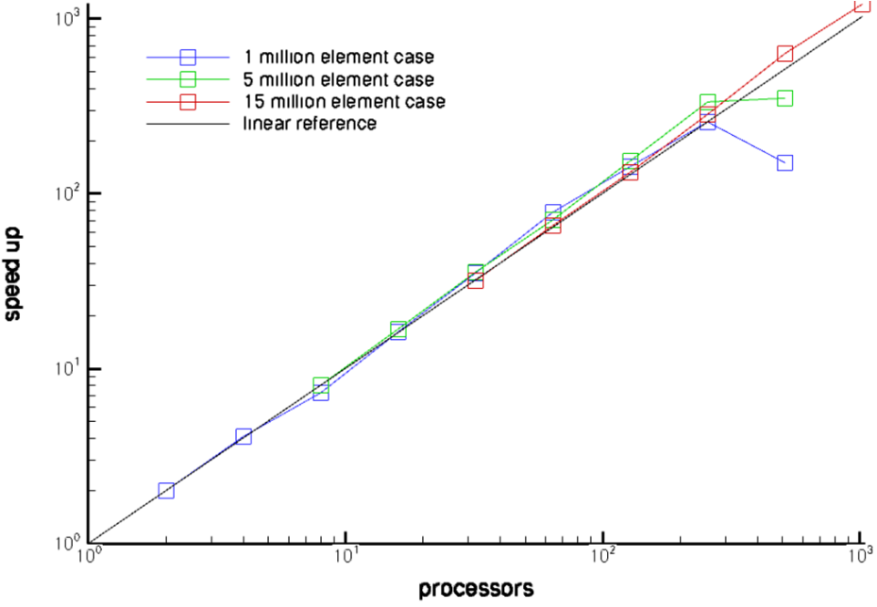
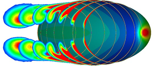
Fig. 1.5.4.1 Demonstration of parallel scalability of Stream: measured speed-up on 3 different mesh sizes for flow over a prolate spheroid at incidence (this case was run on the AFRL HP XC Opteron system).#
stream is routinely run on high-performance computers with parallel architectures – it maintains excellent parallel scalability for grids involving a few million to hundreds of million cells. The plots shown above involve a turbulent flow past a prolate spheroid at an angle of incidence. This case was run on the AFRL HP XC Opteron system (Falcon) at Naval Surface Warfare Center, Panama City, FL (courtesy: Richard Smith). Three different meshes were employed, the finest comprising 15 million nodes. It can be seen that, in this example, stream demonstrates linear scalability up to 1000 processors for the finest mesh.
1.6. References#
S. Balay, K. Buschelman, W. Gropp, D. Kaushik, M. Knepley, L. McInnes, B. Smith, and H. Zhang. Petsc user's manual. Technical Report, Argonne National Laboratory, 2003.
R. Kamakoti, S. Thakur, J. Wright, and W. Shyy. Validation of a new parallel all-speed cfd code in a rule-based framework for multidisciplinary applications. In 36th AIAA Fluid Dynamics Conference and Exhibit. June 2006.
E.A. Luke. Loci: a deductive framework for graph-based algorithms. In S. Matsuoka, R. Oldehoeft, and M. Tholburn, editors, Third International Symposium on Computing in Object-Oriented Parallel Environments, volume 1732 of Lecture Notes in Computer Science, 142–153. Springer-Verlag, Dec. 1999.
E.A. Luke. Loci: a tutorial. Technical Report, Mississippi State University, 2002.
C.C. Nelson and R.H. Nichols. Application of hybrid rans/les turbulence models. In AIAA Paper. 2003.
T. Poinsot and D. Veynante. Theoretical and Numerical Combustion. R.T. Edwards, 2nd edition, 2005.
S. Thakur and J. Wright. An all-speed solver for unsteady reacting and non-reacting flows using a rule-based framework. In 42nd AIAA Fluid Dynamics Conference. 2012.
S. Thakur, J. Wright, and W. Shyy. A pressure-based algorithm for reacting flows with finite rate chemistry. In 34th AIAA Fluid Dynamics Conference. June 2004.
S. Thakur, J. Wright, and W. Shyy. An algorithm for chemically reacting flows on generalized grids using a rule-based framework. In 43rd AIAA Conference. 2005.
F.M. White. Viscous Fluid Flow. McGraw-Hill, 2nd edition, 1991.
D.C. Wilcox. Turbulence Modeling for CFD. DCW Industries, 2nd edition, 2000.
J. Wright and S. Thakur. Development of a pressure-based combustion code in the loci framework. In NASA MSFC Spring Fluids Workshop. April 2004.