4. High-Resolution Schemes for Compressible Flows

In order to accurately predict surface pressure and heat transfer rates in inviscid and viscous compressible flows in an all-speed manner, robust and accurate numerical schemes are required for solving the governing equations. Schemes such as the standard first-order upwind scheme can provide robust solutions for a broad range of flows, but they are not accurate enough in the presence of strong discontinuities such as shock waves. The standard second-order upwind schemes provide relatively accurate results for smooth inviscid and viscous flows, but can cause spurious oscillations near shocks. To remedy these deficiencies, compressible, characteristic-based convection schemes such as AUSM\(^+\)-up, SLAU and SLAU2 schemes have been implemented in Loci-STREAM. These schemes are robust and accurate for inviscid and viscous compressible flows and allow simulations to be performed in an all-speed manner. The AUSM\(^+\)-up scheme and the SLAU2 scheme are robust for flows at all Mach numbers and are relatively simple and accurate. The SLAU2 scheme requires special treatment in unstructured grids to cure the carbuncle phenomenon, which manifests as odd-even decoupling on the shock profile. The hybrid-SLAU2 scheme is designed to resolve the carbuncle phenomenon in hypersonic flows on unstructured grids. The convergence properties of different convection schemes and limiters are examined for a variety of test cases.

4.1. AUSM±up for Unstructured Grids

The AUSM\(^+\) scheme, originally developed by Liou [38], is an improvement over the earlier AUSM scheme developed by Liou and Steffen [39]. Like AUSM, AUSM\(^+\) is based on splitting of inviscid fluxes into convective and pressure parts. The improvement in AUSM\(^+\) is in the Mach-number based splitting, which is defined as a third-order polynomial in the subsonic region with higher-order dissipation terms. The AUSM\(^+\)-up scheme is a pressure- and velocity-corrected version of AUSM\(^+\).

Consider the one-dimensional Euler equations in conservative form:

(4.1.1)\[\frac{\partial \mathbf{W}}{\partial t} + \frac{\partial \mathbf{F}}{\partial x} = 0\]

where the conserved-variable vector and inviscid flux vector are

(4.1.2)\[\begin{split}\mathbf{W} = \begin{pmatrix} \rho\\ \rho u\\ \rho E \end{pmatrix}, \qquad \mathbf{F} = \begin{pmatrix} \rho u\\ \rho u^2 + p\\ \rho H u \end{pmatrix}.\end{split}\]

Here, \(E\) is the total energy, \(E = r\left(e + u^2/2\right)\), and \(H = E + p\) is the total enthalpy.

The AUSM-family methods split the flux into convective and pressure parts:

(4.1.3)\[\begin{split}\mathbf{F}=\mathbf{F}^c+\mathbf{F}^p = \begin{pmatrix} \rho u\\ m u\\ H u \end{pmatrix} + \begin{pmatrix} 0\\ p\\ 0 \end{pmatrix}.\end{split}\]

At a face (interface) \(f\), the numerical flux is written as

(4.1.4)\[\mathbf{F}_f = \dot{m}_f\,\boldsymbol{\Phi}_f + p_f.\]

with

(4.1.5)\[\begin{split}\boldsymbol{\Phi}= \begin{pmatrix} 1\\ u\\ H \end{pmatrix}.\end{split}\]

and the upwinding rule

(4.1.6)\[\begin{split}\boldsymbol{\Phi}_f= \begin{cases} \boldsymbol{\Phi}_L,& \dot{m}_f>0,\\ \boldsymbol{\Phi}_R,& \text{otherwise}. \end{cases}\end{split}\]

4.1.1. Mass flux

The left/right Mach numbers are defined as

(4.1.1.1)\[M_{L/R}=\frac{u_{L/R}}{a_{1/2}},\]

with face-averaged sound speed

(4.1.1.2)\[a_{1/2}=\frac{1}{2}\left(a_L+a_R\right).\]

Define

(4.1.1.3)\[\bar{M}^{2}=\frac{u_L^2+u_R^2}{2a_f^2},\]

(4.1.1.4)\[M_0^2=\min\!\left(1,\max\!\left(\bar{M}^2,M_\infty^2\right)\right)\in[0,1],\]

(4.1.1.5)\[f_a(M_0)=M_0(2-M_0)\in[0,1].\]

The interface Mach number used by AUSM\(^+\)-up is

(4.1.1.6)\[M_f=\mathcal{M}_{(4)}^{+}(M_L)+\mathcal{M}_{(4)}^{-}(M_R) -\frac{K_p}{f_a}\max\!\left(1-\sigma \bar{M}^2,0\right) \frac{p_R-p_L}{\rho_{1/2}a_{1/2}^2}.\]

with

(4.1.1.7)\[\rho_{1/2}=\frac{1}{2}\left(\rho_L+\rho_R\right).\]

where \(0 \le K_p \le 1\) and \(\sigma \le 1\).

The Mach-number splitting function is

(4.1.1.8)\[\begin{split}\mathcal{M}_{(4)}^{\pm}(M)= \begin{cases} \mathcal{M}_{(1)}^{\pm}, & |M|\ge 1,\\[4pt] \mathcal{M}_{(2)}^{\pm}\left(1\mp 16\beta\,\mathcal{M}_{(2)}^{\mp}\right), & \text{otherwise}, \end{cases}\end{split}\]

where

(4.1.1.9)\[\mathcal{M}_{(1)}^{\pm}(M)=\frac{1}{2}\left(M\pm |M|\right), \qquad \mathcal{M}_{(2)}^{\pm}(M)=\pm \frac{1}{4}(M\pm 1)^2.\]

The face mass flux is

(4.1.1.10)\[\begin{split}\dot{m}_{1/2}=M_{1/2}a_{1/2} \begin{cases} \rho_L, & M_{1/2}\ge 0,\\ \rho_R, & \text{otherwise}. \end{cases}\end{split}\]

4.1.2. Pressure Flux

The face pressure is computed as

(4.1.2.1)\[p_f=\mathcal{P}_{(5)}^{+}(M_L)p_L+\mathcal{P}_{(5)}^{-}(M_R)p_R -K_u\,\mathcal{P}_{(5)}^{+}(M_L)\mathcal{P}_{(5)}^{-}(M_R)(\rho_L+\rho_R)(f_a a_{1/2})(u_R-u_L).\]

The splitting of pressure can be achieved in a manner similar to the van Leer splitting for the fluxes of the Euler equations. The van Leer splitting is based on the requirements that the split fluxes as well as their first-derivatives be continuous and that the split fluxes be polynomials of the lowest possible degree. This leads to a splitting of the fluxes in terms of factors \( (M\pm 1)^2 \). The following splitting is employed:

(4.1.2.2)\[\begin{split}\mathcal{P}_{(5)}^{\pm}(M)= \begin{cases} \dfrac{1}{M}\mathcal{M}_{(1)}^{\pm}, & |M|\ge 1,\\[6pt] \mathcal{M}_{(2)}^{\pm}\left[(\pm 2-M)\mp 16\alpha M\,\mathcal{M}_{(2)}^{\mp}\right], & \text{otherwise}. \end{cases}\end{split}\]

with parameters

(4.1.2.3)\[\alpha=\frac{3}{16}\left(-4+5f_a^2\right)\in\left[-\frac{3}{4},\frac{3}{16}\right], \qquad \beta=\frac{1}{8}.\]

and \(0\le K_u \le 1\). Thus, for supersonic flow, the above formulation leads to full upwinding of pressure:

(4.1.2.4)\[p_f=p_L \quad \text{if } |M|>1 \text{ and } M>0.\]

The splitting takes place only for subsonic flow, where contributions from both upwind and downwind sides are present:

(4.1.2.5)\[p_f= \left[\frac{1}{4}(M_L+1)^2(2-M_L)+\alpha M_L(M_L^2-1)^2\right]p_L + \left[\frac{1}{4}(M_R-1)^2(2+M_R)-\alpha M_R(M_R^2-1)^2\right]p_R.\]

4.1.3. AUSM±up Momentum Equation

The discretized momentum equation can be written as

(4.1.3.1)\[\left(a_0+\frac{\rho_0^n\Omega_0}{\Delta t}\right)\mathbf{V}_0 = \sum a_{\mathrm{nbr}0}\mathbf{V}_{\mathrm{nbr}} +\hat{\mathbf{b}}_0 -\sum_f (p_f\mathbf{A})_0 +\frac{\rho_0^n\Omega_0}{\Delta t}\mathbf{V}_0^n.\]

or

(4.1.3.2)\[a_0^T\mathbf{V}_0 = \sum a_{\mathrm{nbr}0}\mathbf{V}_{\mathrm{nbr}} +\hat{\mathbf{b}}_0 -\sum_f (p_f\mathbf{A})_0 +\frac{\rho_0^n\Omega_0}{\Delta t}\mathbf{V}_0^n,\]

with

(4.1.3.3)\[a_0^T=a_0+\frac{\rho_0^n\Omega_0}{\Delta t}, \qquad a_0=\sum a_{\mathrm{nbr}0}.\]

Applying under-relaxation yields

(4.1.3.4)\[a_0^T\mathbf{V}_0^{k+1} = \alpha\!\left[ \sum a_{\mathrm{nbr}0}\mathbf{V}_{\mathrm{nbr}}^{k+1} +\hat{\mathbf{b}}_0 -\sum_f(p_f\mathbf{A})_0 +\frac{\rho_0^n\Omega_0}{\Delta t}\mathbf{V}_0^n \right] +(1-\alpha)a_0^T\mathbf{V}_0^k.\]

which is equivalent to

(4.1.3.5)\[\frac{a_0^T}{\alpha}\mathbf{V}_0^{k+1} = \sum a_{\mathrm{nbr}0}\mathbf{V}_{\mathrm{nbr}}^{k+1} +\hat{\mathbf{b}}_0 -\sum_f(p_f\mathbf{A})_0 +\frac{\rho_0^n\Omega_0}{\Delta t}\mathbf{V}_0^n +(1-\alpha)\frac{a_0^T}{\alpha}\mathbf{V}_0^k.\]

and finally

(4.1.3.6)\[\mathbf{V}_0^{k+1} = \alpha\!\left[ \frac{\sum a_{\mathrm{nbr}0}\mathbf{V}_{\mathrm{nbr}}^{k+1}+\hat{\mathbf{b}}_0}{a_0^T} -\frac{\sum_f(p_f\mathbf{A})_0}{a_0^T} +\frac{\rho_0^n\Omega_0}{a_0^T\Delta t}\mathbf{V}_0^n \right] +(1-\alpha)\mathbf{V}_0^k.\]

4.1.4. AUSM±up Pressure Correction Equation

The mass flux at a face is

(4.1.4.1)\[\dot{m}_f=\rho_f M_f a_f A_f.\]

4.1.5. Option 1

For unstructured grids, one option is to include the pressure correction term inside \(\dot{m}\):

(4.1.5.1)\[\dot{m}_{1/2} = \rho_{1/2} \left[ \mathcal{M}_{(4)}^{+}(M_L)+\mathcal{M}_{(4)}^{-}(M_R) -\frac{K_p}{f_a}\max(1-\sigma\bar{M}^2,0)\frac{p_R-p_L}{\rho_{1/2}a_{1/2}^2} \right] a_{1/2}A_f.\]

The pressure-correction contribution is then

(4.1.5.2)\[\dot{m}_{1/2}' = -\rho_{1/2} \left[ \frac{K_p}{f_a}\max(1-\sigma\bar{M}^2,0)\frac{p_R-p_L}{\rho_{1/2}a_{1/2}^2} \right] a_{1/2}A_f = -\frac{K_p}{f_a}\max(1-\sigma\bar{M}^2,0)\frac{(p_R'-p_L')}{a_{1/2}}A_f.\]

The continuity equation is written as

(4.1.5.3)\[\frac{\Delta\rho}{\Delta t}\Omega + \sum_f \left(\dot{m}_f^*+\dot{m}_f'\right)=0.\]

with

(4.1.5.4)\[\Delta\rho=\rho^{k+1}-\rho^n =(\rho^{k+1}-\rho^k)-(\rho^k-\rho^n) =\rho' + (\rho^k-\rho^n).\]

and (using the ideal-gas relation)

(4.1.5.5)\[\frac{\Delta\rho}{\Delta t} =\frac{1}{\Delta t}\left[\frac{p'}{\gamma RT}+(\rho^k-\rho^n)\right].\]

4.1.6. Option 2

(Not provided in the source PDF. Add your implementation notes here.)

4.2. Simple Low-Dissipation AUSM (SLAU) Scheme

SLAU(2) (Simple Low-dissipation AUSM, version 2) is another AUSM-family method for compressible flows. In 3D it is written as

(4.2.1)\[\mathbf{F}_{\mathrm{SLAU(2)}}=\dot{m}_f\boldsymbol{\Phi}_f+p_f\mathbf{N}.\]

where

(4.2.2)\[\begin{split}\boldsymbol{\Phi}= \begin{pmatrix} 1\\ u\\ v\\ w\\ H \end{pmatrix}, \qquad \mathbf{N}= \begin{pmatrix} 0\\ n_x\\ n_y\\ n_z\\ 0 \end{pmatrix}.\end{split}\]

and

(4.2.3)\[\begin{split}\boldsymbol{\Phi}_f= \begin{cases} \boldsymbol{\Phi}_L,& \dot{m}_f>0,\\ \boldsymbol{\Phi}_R,& \text{otherwise}. \end{cases}\end{split}\]

Equivalently, the flux can be expanded as

(4.2.4)\[\mathbf{F}_{\mathrm{SLAU(2)}}= \left(\frac{\dot{m}_f+|\dot{m}_f|}{2}\right)\boldsymbol{\Phi}_L +\left(\frac{\dot{m}_f-|\dot{m}_f|}{2}\right)\boldsymbol{\Phi}_R +p_f\mathbf{N}.\]

The SLAU(2) mass flux is

(4.2.5)\[\left(\dot{m}_f\right)_{\mathrm{SLAU(2)}} = \frac{1}{2}\left\{ \rho_L\left(V_{nL}+|\bar{V}_n|^{+}\right) +\rho_R\left(V_{nR}-|\bar{V}_n|^{-}\right) -\frac{\chi}{\bar{c}}\Delta p \right\}.\]

with

(4.2.6)\[|\bar{V}_n|^{+}=(1-g)|\bar{V}_n|+g|V_{nL}|, \qquad |\bar{V}_n|^{-}=(1-g)|\bar{V}_n|+g|V_{nR}|.\]

(4.2.7)\[|\bar{V}_n| =\frac{\rho_L|V_{nL}|+\rho_R|V_{nR}|}{\rho_L+\rho_R}.\]

(4.2.8)\[g=-\max\!\left[\min(M_L,0),-1\right]\, \min\!\left[\max(M_R,0),1\right].\]

(4.2.9)\[\chi=(1-\bar{M})^2.\]

(4.2.10)\[\bar{M}=\min\!\left(1,\frac{1}{\bar{c}}\sqrt{\frac{u_L^2+u_R^2}{2}}\right), \qquad M=\frac{V_n}{\bar{c}}=\frac{\mathbf{u}\cdot\mathbf{n}}{\bar{c}}, \qquad \bar{c}=\frac{c_L+c_R}{2}.\]

4.2.1. Face pressure (SLAU / SLAU2)

The SLAU face pressure is

(4.2.1.1)\[(p_f)_{\mathrm{SLAU}} = \frac{p_L+p_R}{2} +\frac{f^{+}(M_L)-f^{-}(M_R)}{2}(p_L-p_R) +\left(f^{+}(M_L)+f^{-}(M_R)-1\right)(1-\chi)\frac{p_L+p_R}{2}.\]

The SLAU2 face pressure is

(4.2.1.2)\[(p_f)_{\mathrm{SLAU2}} = \frac{p_L+p_R}{2} +\frac{f^{+}(M_L)-f^{-}(M_R)}{2}(p_L-p_R) +\left(f^{+}(M_L)+f^{-}(M_R)-1\right)\sqrt{\frac{u_L^2+u_R^2}{2}}\,\bar{\rho}\bar{c}.\]

where

(4.2.1.3)\[\bar{\rho}=\frac{\rho_L+\rho_R}{2}.\]

and

(4.2.1.4)\[\begin{split}f^{\pm}(M)= \begin{cases} \dfrac{1}{2}\left(1\pm \mathrm{sign}(M)\right), & |M|\ge 1,\\[6pt] \dfrac{1}{4}(M\pm 1)^2(2\mp M), & \text{otherwise}. \end{cases}\end{split}\]

Implementation notes (from the source PDF):

• Options:

  1. Use \((p_f)_{\mathrm{SLAU}}\) with \((\dot{m}_f)_{\mathrm{SLAU}}\).

  2. Use \((p_f)_{\mathrm{SLAU2}}\) with \((\dot{m}_f)_{\mathrm{SLAU}}\).

• The SLAU2 scheme uses the same \((\dot{m}_f)_{\mathrm{SLAU}}\) from the SLAU scheme, while \((p_f)_{\mathrm{SLAU2}}\) incorporates the velocity magnitude for stabilizing shock waves.

• \(\dot{m}_{f,\mathrm{SLAU2}} \equiv \dot{m}_{f,\mathrm{SLAU}}\).

4.3. SLAU/SLAU2 Momentum Equation

The (discretized) momentum equation is

(4.3.1)\[\left(a_0+\frac{\rho_0^n\Omega_0}{\Delta t}\right)\mathbf{V}_0 = \sum a_{\mathrm{nbr}0}\mathbf{V}_{\mathrm{nbr}} +\hat{\mathbf{b}}_0 -\sum_f (p_f\mathbf{A})_0 +\frac{\rho_0^n\Omega_0}{\Delta t}\mathbf{V}_0^n.\]

(4.3.2)\[a_0^T\mathbf{V}_0 = \sum a_{\mathrm{nbr}0}\mathbf{V}_{\mathrm{nbr}} +\hat{\mathbf{b}}_0 -\sum_f (p_f\mathbf{A})_0 +\frac{\rho_0^n\Omega_0}{\Delta t}\mathbf{V}_0^n.\]

(4.3.3)\[a_0^T=a_0+\frac{\rho_0^n\Omega_0}{\Delta t}, \qquad a_0=\sum a_{\mathrm{nbr}0}.\]

(4.3.4)\[a_0^T\mathbf{V}_0^{k+1} = \alpha\!\left[ \sum a_{\mathrm{nbr}0}\mathbf{V}_{\mathrm{nbr}}^{k+1} +\hat{\mathbf{b}}_0 -\sum_f(p_f\mathbf{A})_0 +\frac{\rho_0^n\Omega_0}{\Delta t}\mathbf{V}_0^n \right] +(1-\alpha)a_0^T\mathbf{V}_0^k.\]

(4.3.5)\[\frac{a_0^T}{\alpha}\mathbf{V}_0^{k+1} = \sum a_{\mathrm{nbr}0}\mathbf{V}_{\mathrm{nbr}}^{k+1} +\hat{\mathbf{b}}_0 -\sum_f(p_f\mathbf{A})_0 +\frac{\rho_0^n\Omega_0}{\Delta t}\mathbf{V}_0^n +(1-\alpha)\frac{a_0^T}{\alpha}\mathbf{V}_0^k.\]

(4.3.6)\[\mathbf{V}_0^{k+1} = \alpha\!\left[ \frac{\sum a_{\mathrm{nbr}0}\mathbf{V}_{\mathrm{nbr}}^{k+1}+\hat{\mathbf{b}}_0}{a_0^T} -\frac{\sum_f(p_f\mathbf{A})_0}{a_0^T} +\frac{\rho_0^n\Omega_0}{a_0^T\Delta t}\mathbf{V}_0^n \right] +(1-\alpha)\mathbf{V}_0^k.\]

4.4. SLAU/SLAU2 Pressure Correction Equation

Substituting Eq. (2.40) into Eq. (2.37) yields

(4.4.1)\[\left(\dot{m}_f\right)_{\mathrm{SLAU}} = \frac{1}{2}\left\{ \rho_L\left(V_{nL}+|\bar{V}_n|^{+}\right) +\rho_R\left(V_{nR}-|\bar{V}_n|^{-}\right) -\frac{\chi}{\bar{c}}(p_R-p_L) \right\}A_f.\]

with the pressure-correction part

(4.4.2)\[\dot{m}_f'=-\frac{\chi}{\bar{c}}(p_R'-p_L')A_f.\]

Using the discretized continuity equation,

(4.4.3)\[\frac{\Delta\rho}{\Delta t}\Omega + \sum_f\left(\dot{m}_f^*+\dot{m}_f'\right)=0,\]

and

(4.4.4)\[\Delta\rho=\rho^{k+1}-\rho^n =(\rho^{k+1}-\rho^k)-(\rho^k-\rho^n) =\rho' + (\rho^k-\rho^n),\]

together with

(4.4.5)\[\frac{\Delta\rho}{\Delta t} =\frac{1}{\Delta t}\left[\frac{p'}{\gamma RT}+(\rho^k-\rho^n)\right],\]

the pressure correction equation is

(4.4.6)\[a_0 p_0'=\sum_{\mathrm{nbr}} a_{\mathrm{nbr}}p_{\mathrm{nbr}}' + b.\]

The neighbor coefficients are

(4.4.7)\[a_{\mathrm{nbr}} = \frac{(\rho A\Omega)_f}{(\mathbf{r}_1-\mathbf{r}_0)\cdot\hat{\mathbf{n}}} \left(\frac{1}{a_0^{u}}+\frac{1}{a_1^{u}}\right).\]

with

(4.4.8)\[a_0=\sum_{\mathrm{nbr}} a_{\mathrm{nbr}}.\]

and the source term

(4.4.9)\[b=-\sum_f \dot{m}_f^{*}.\]

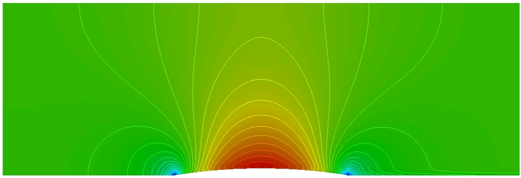
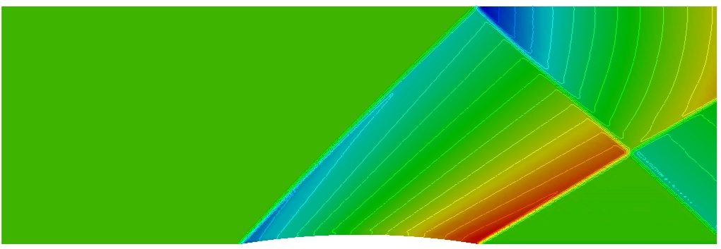
Fig. 4.4.1 Mach number contours for flow over a bump using the AUSM+ scheme: subsonic (top) and supersonic (bottom).

4.5. Standard Limiters: Barth-Jespersen (BJ) and Venkatakrishnan (V)

This section summarizes common slope limiters used to prevent spurious oscillations near discontinuities while maintaining second-order accuracy where possible.

For a face \(k\) between cells \(i\) and \(j\), the limited reconstructions are

(4.5.1)\[q_k^{+}=q_i+\phi_i\nabla q_i\cdot \Delta r_{ik},\]

(4.5.2)\[q_k^{-}=q_j+\phi_j\nabla q_j\cdot \Delta r_{jk}.\]

The BJ/V limiter factor is computed as

(4.5.3)\[\begin{split}\phi_i^{\mathrm{BJ/V}}= \min_{\text{overall }t\text{ values}} \begin{cases} f^{\mathrm{BJ/V}}\!\left(\dfrac{q_i^{\max}-q_i}{q_t-q_i}\right), & q_t-q_i>0,\\[10pt] f^{\mathrm{BJ/V}}\!\left(\dfrac{q_i^{\min}-q_i}{q_t-q_i}\right), & q_t-q_i<0,\\[10pt] 1, & q_t-q_i=0, \end{cases}\end{split}\]

where the BJ limiter uses

(4.5.4)\[f^{\mathrm{BJ}}\!\left(\frac{a}{b}\right)=\min\!\left(1,\frac{a}{b}\right),\]

and the Venkatakrishnan limiter uses

(4.5.5)\[f^{\mathrm{V}}\!\left(\frac{a}{b}\right) = \frac{1}{b} \left( \frac{(a^2+\epsilon^2)b+2b^2a}{a^2+2b^2+ab+\epsilon^2} \right).\]

with

(4.5.6)\[\epsilon^2=(K\Delta h)^3.\]

The cellwise bounds are

(4.5.7)\[q_i^{\max}=\max\!\left[q_i,\max_{j\in V(i)}(q_j)\right],\]

(4.5.8)\[q_i^{\min}=\min\!\left[q_i,\min_{j\in V(i)}(q_j)\right].\]

and the limiter enforces

(4.5.9)\[q_i^{\min}\le q_t\le q_i^{\max}.\]

The “test values” are defined as:

(4.5.10)\[q_t^{(v)}=q_i+\nabla q_i\cdot \Delta r_{il}, \qquad l\in v(i),\]

(4.5.11)\[q_t^{(f)}=q_i+\nabla q_i\cdot \Delta r_{ik}, \qquad \partial\Omega_k\subset \partial\Omega_i.\]

4.6. Multidimensional Limiters

This section discusses multidimensional limiting strategies, including the MLP and MLP-pw limiters for unstructured grids.

4.6.1. Brief Review of Barth-Jespersen and Venkatakrishnan Limiters

The limited face reconstructions are

(4.6.1.1)\[q_k^{+}=q_i+\psi_i\nabla q_i\cdot \Delta r_{ik}, \qquad q_k^{-}=q_j+\psi_j\nabla q_j\cdot \Delta r_{jk}.\]

The limiter coefficient is computed as

(4.6.1.2)\[\begin{split}\psi_i^{\mathrm{BJ/V}}= \min_{\text{overall }t\text{ values}} \begin{cases} f_{\mathrm{BJ/V}}\!\left(\dfrac{q_i^{\max}-q_i}{q_t-q_i}\right), & q_t-q_i>0,\\[10pt] f_{\mathrm{BJ/V}}\!\left(\dfrac{q_i^{\min}-q_i}{q_t-q_i}\right), & q_t-q_i<0,\\[10pt] 1, & q_t-q_i=0, \end{cases}\end{split}\]

The BJ function is

(4.6.1.3)\[f_{\mathrm{BJ}}\!\left(\frac{\Delta_+}{\Delta_-}\right)=\min\!\left(1,\frac{\Delta_+}{\Delta_-}\right),\]

where \(\Delta_+=q^{\max,\min}-q_i\) and \(\Delta_-=\phi_t-\phi_i\) (as stated in the source PDF).

The Venkatakrishnan-type function is

(4.6.1.4)\[f_{\mathrm{V}}\!\left(\frac{\Delta_+}{\Delta_-}\right) = \frac{1}{\Delta_-} \left( \frac{(\Delta_+^2+\epsilon^2)\Delta_-+2\Delta_-^2\Delta_+}{\Delta_+^2+2\Delta_-^2+\Delta_+\Delta_-+\epsilon^2} \right).\]

with

(4.6.1.5)\[\epsilon^2=(K\Delta h)^3.\]

The bounds and test values used are

(4.6.1.6)\[q_i^{\max}=\max\!\left[q_i,\max_{j\in V(i)}(q_j)\right], \qquad q_i^{\min}=\min\!\left[q_i,\min_{j\in V(i)}(q_j)\right].\]

(4.6.1.7)\[q_i^{\min}\le q_t\le q_i^{\max}.\]

(4.6.1.8)\[q_t^{(v)}=q_i+\nabla q_i\cdot \Delta r_{il}, \qquad l\in v(i),\]

(4.6.1.9)\[q_t^{(f)}=q_i+\nabla q_i\cdot \Delta r_{if}, \qquad \partial\Omega_f\subset \partial\Omega_i.\]

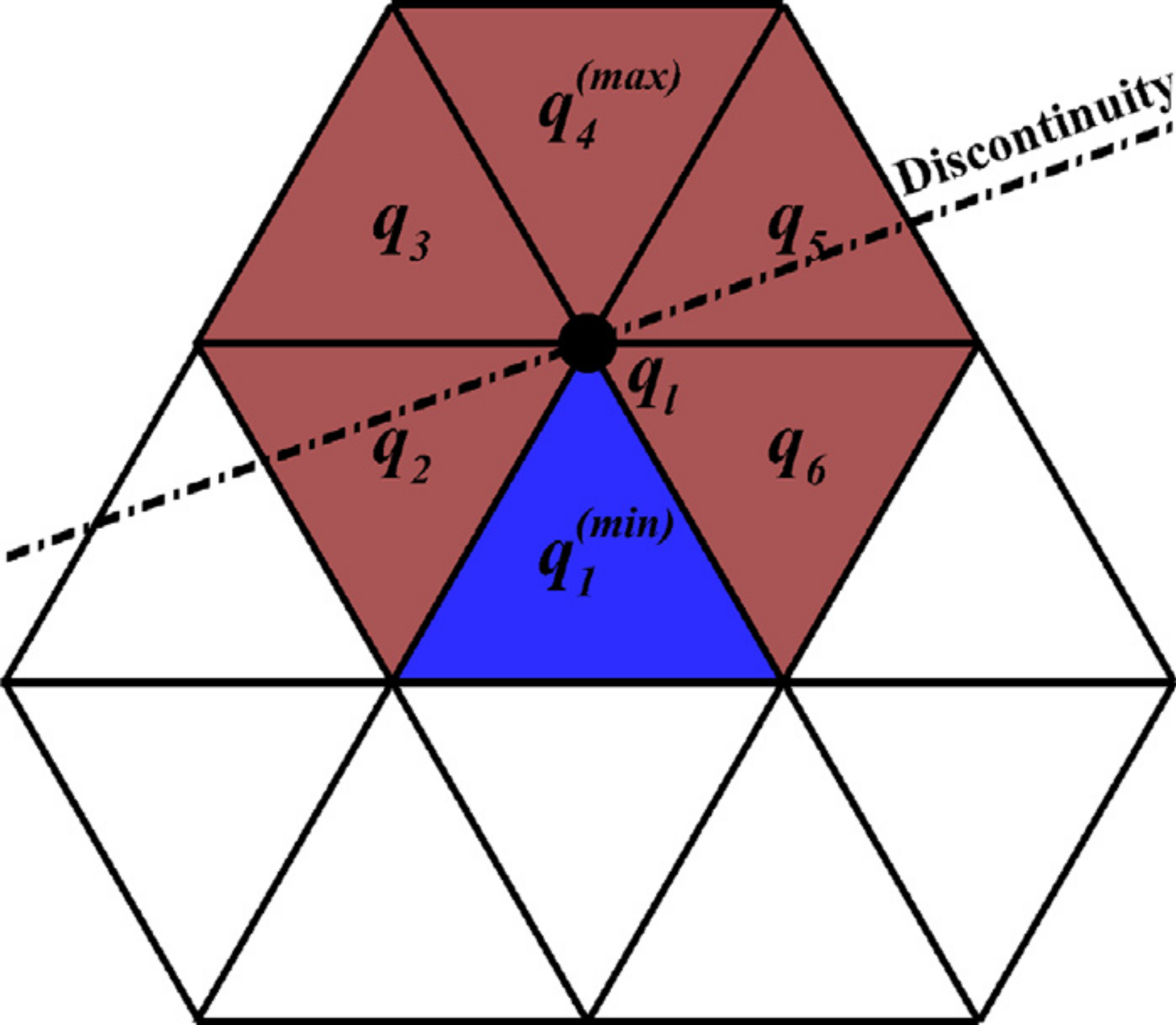
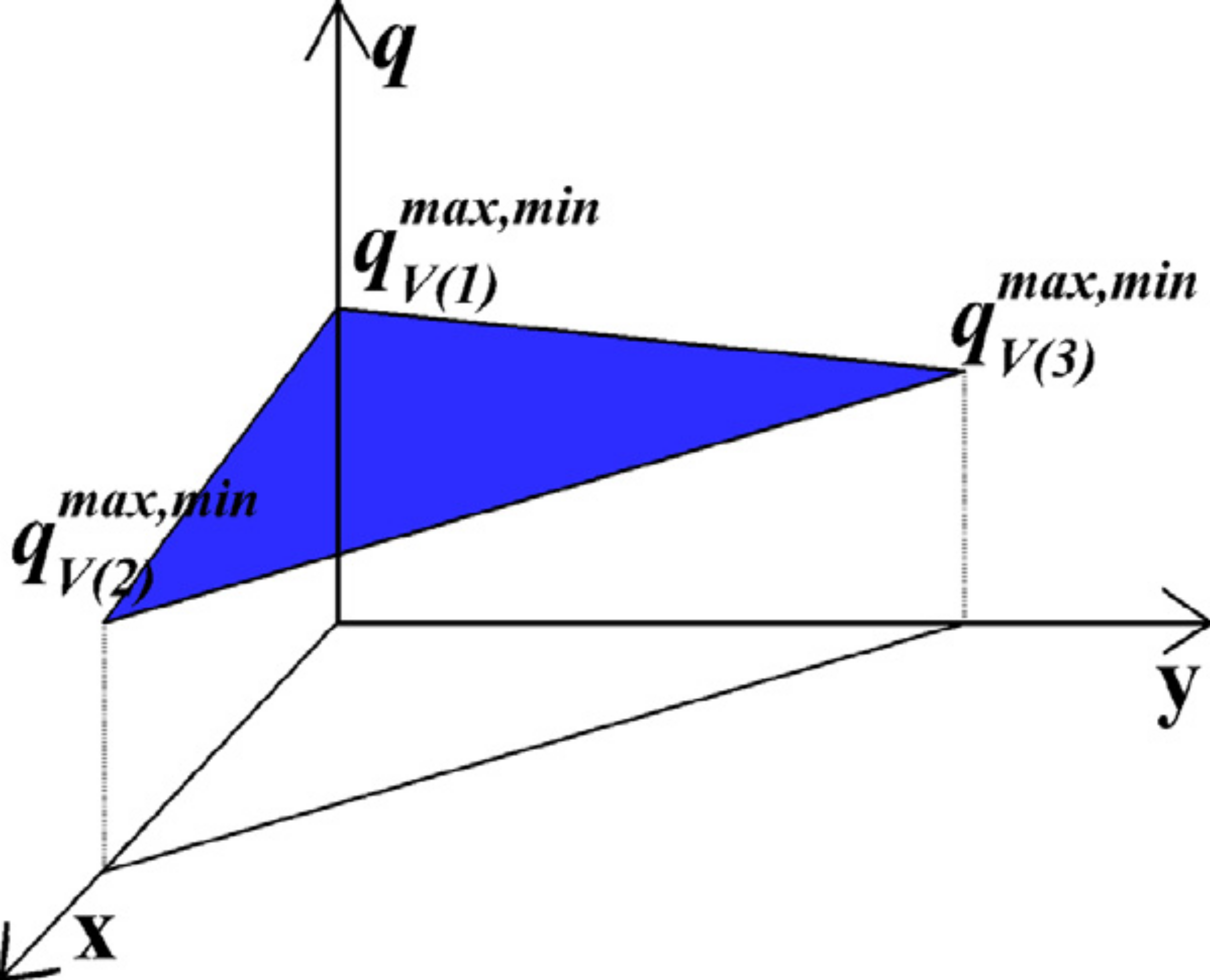
Fig. 4.6.1.1 Schematic diagrams of the unstructured MLP limiter.

4.6.2. Unstructured MLP Limiter

To satisfy monotonicity, the reconstructed values at vertices must remain in the bounds computed from vertex neighborhoods:

(4.6.2.1)\[q_{V(l)}^{\min}\le q_l \le q_{V(l)}^{\max}, \qquad l\in v(i).\]

where the unlimited vertex reconstruction is

(4.6.2.2)\[q_l = q_i + \nabla q_i\cdot \Delta r_{il},\]

and the vertex bounds are

(4.6.2.3)\[q_{V(l)}^{\max}=\max_{j\in V(l)}(q_j), \qquad q_{V(l)}^{\min}=\min_{j\in V(l)}(q_j).\]

This yields an admissible range for \(\psi_l\):

(4.6.2.4)\[\frac{q_{V(l)}^{\min}-q_i}{\nabla q\cdot \Delta r_{il}} \le \psi_l \le \frac{q_{V(l)}^{\max}-q_i}{\nabla q\cdot \Delta r_{il}}.\]

The MLP condition is summarized as

(4.6.2.5)\[q_{v(i)}^{\min,n}\le q_i^{n+1}\le q_{v(i)}^{\max,n}.\]

where

(4.6.2.6)\[q_{v(i)}^{\max}=\max_{l\in v(i)}\!\left(q_{V(l)}^{\max}\right), \qquad q_{v(i)}^{\min}=\min_{l\in v(i)}\!\left(q_{V(l)}^{\min}\right).\]

The limiter coefficient is then

(4.6.2.7)\[\begin{split}\psi_i^{\mathrm{MLP}} = \min_{l\in v(i)} \begin{cases} f_{\mathrm{MLP}}\!\left(\dfrac{q_{V(l)}^{\max}-q_i}{q_l-q_i}\right), & q_l-q_i>0,\\[10pt] f_{\mathrm{MLP}}\!\left(\dfrac{q_{V(l)}^{\min}-q_i}{q_l-q_i}\right), & q_l-q_i<0,\\[10pt] 1, & q_l-q_i=0, \end{cases}\end{split}\]

where \(f_{\mathrm{MLP}}\) can be chosen as either \(f_{\mathrm{BJ}}\) or \(f_{\mathrm{V}}\).

4.6.3. Unstructured MLP-pw limiter

An averaged (piecewise) vertex bound is defined by

(4.6.3.1)\[\bar{q}_k^{\max}=\frac{\sum_{l\in v(k)} q_{V(l)}^{\max}}{n_{v(k)}}, \qquad \bar{q}_k^{\min}=\frac{\sum_{l\in v(k)} q_{V(l)}^{\min}}{n_{v(k)}}.\]

and the reconstructed interface values satisfy

(4.6.3.2)\[\bar{q}_k^{\min}\le q_k^{\pm}\le \bar{q}_k^{\max}.\]

The “weak-MLP” constraint is

(4.6.3.3)\[\bar{q}_{v(i)}^{\min}\le q \le \bar{q}_{v(i)}^{\max}.\]

with

(4.6.3.4)\[\bar{q}_{v(i)}^{\min}=\min_{l\in v(i)}\left(\bar{q}_l\right), \qquad \bar{q}_{v(i)}^{\max}=\max_{l\in v(i)}\left(\bar{q}_l\right).\]

The averaged vertex value is computed via weighted averaging:

(4.6.3.5)\[\bar{q}_l=\frac{\sum_{i\in V(l)}\omega_{li}q_i}{\sum_{i\in V(l)}\omega_{li}}, \qquad \omega_{li}\ge 0.\]

A simple choice is inverse-distance weights:

(4.6.3.6)\[\omega_{li}=\frac{1}{\left|\Delta r_{li}\right|}.\]

4.6.3.1. Pressure Weight Function

A pressure weight function is defined as

(4.6.3.7)\[\omega_p=\left(\frac{\bar{p}_{v(i)}^{\min}}{\bar{p}_{v(i)}^{\max}}\right)^3,\]

where

(4.6.3.8)\[\bar{p}_{v(i)}^{\max}=\max_{l\in v(i)}\left(\bar{p}_l\right), \qquad \bar{p}_{v(i)}^{\min}=\min_{l\in v(i)}\left(\bar{p}_l\right).\]

The MLP-pw limiter is expressed as

(4.6.3.9)\[\begin{split}\psi_i^{\mathrm{MLP\text{-}pw}} = \min_{l\in v(i)} \begin{cases} f_{\mathrm{MLP}}\!\left(\dfrac{\omega_p \bar{q}_k^{\max}+(1-\omega_p)\bar{q}_{v(i)}^{\max}-q_i}{q_k-q_i}\right), & q_k-q_i>0,\\[10pt] f_{\mathrm{MLP}}\!\left(\dfrac{\omega_p \bar{q}_k^{\min}+(1-\omega_p)\bar{q}_{v(i)}^{\min}-q_i}{q_k-q_i}\right), & q_k-q_i<0,\\[10pt] 1, & q_k-q_i=0, \end{cases}\end{split}\]

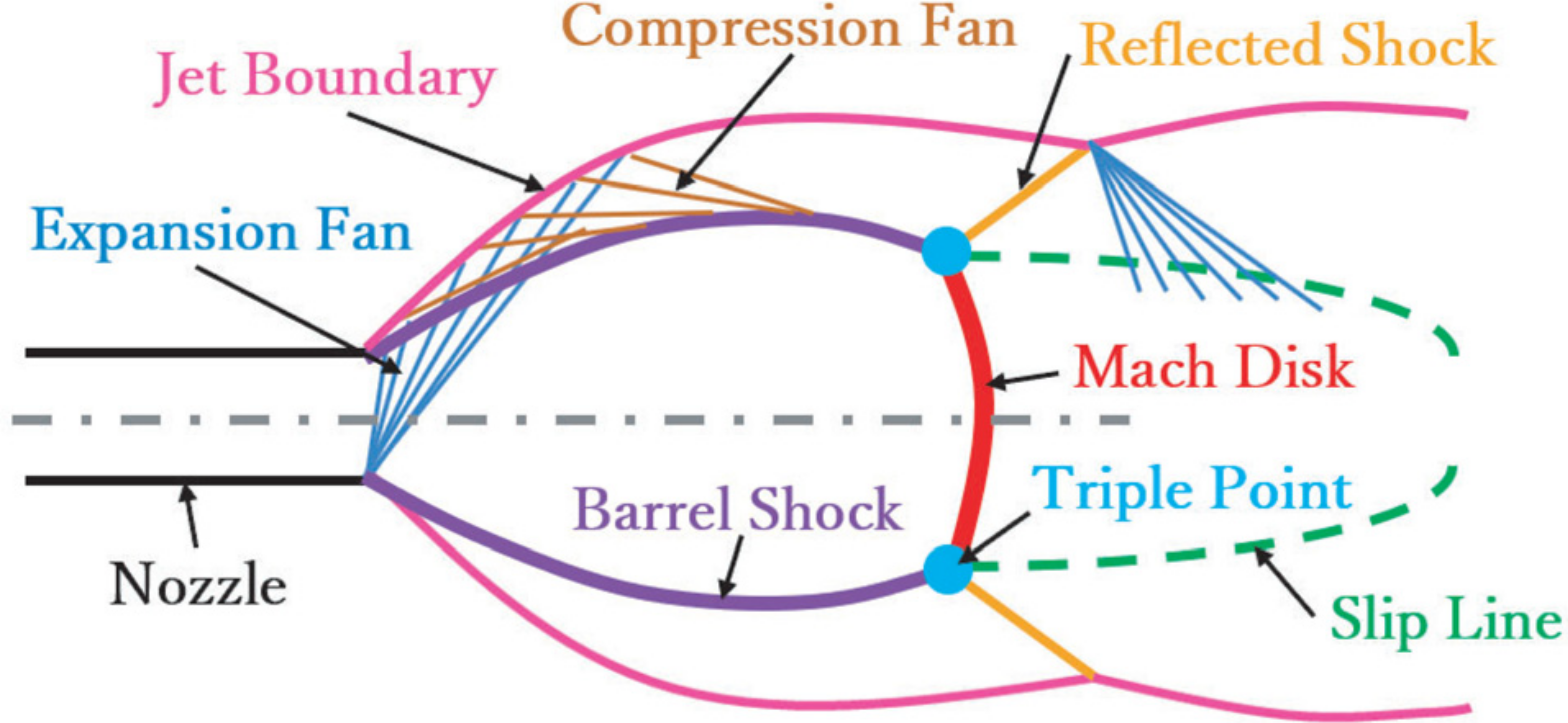
Fig. 4.6.3.1 Key flow features including Mach disk in an under-expanded jet.

4.7. Hybrid SLAU/SLAU2 Backends (van Leer, HLLE, HLLEM, LM-HLLEM, HLLEMCC)

In Loci-STREAM, hybrid SLAU/SLAU2 augments the SLAU momentum dissipation with a backend dissipation model to improve robustness near strong shocks while preserving low-dissipation behavior away from shocks.

For each face, define the SLAU dissipation magnitude used by the momentum source assembly as

(4.7.1)\[\Delta m_f^{\mathrm{SLAU}} = \left|\rho_f\left(V_f-V_{g,f}\right)\right|,\]

where \(\rho_f\) is face density, \(V_f\) is face volume flux, and \(V_{g,f}\) is grid volume flux.

The cell-level pressure weight is

(4.7.2)\[\omega_{p,i} = \left(\frac{p_{v(i)}^{\min}}{p_{v(i)}^{\max}}\right)^3,\]

and the face value is

(4.7.3)\[\omega_{p,f}=\min\!\left(\omega_{p,L},\omega_{p,R}\right).\]

The hybrid dissipation magnitude is then

(4.7.4)\[\Delta m_f^{\mathrm{hyb}} = \left(1-\omega_{p,f}\right)\Delta m_f^{B} +\omega_{p,f}\Delta m_f^{\mathrm{SLAU}},\]

where \(\Delta m_f^{B}\) is from the selected backend \(B\).

The added hybrid momentum source vector is

(4.7.5)\[\mathbf{S}_f^{\mathrm{hyb}} = \frac{1}{2}\left(\Delta m_f^{\mathrm{hyb}}-\Delta m_f^{\mathrm{SLAU}}\right) \left(\mathbf{u}_L-\mathbf{u}_R\right).\]

This source is assembled antisymmetrically on the two adjacent cells:

(4.7.6)\[\mathbf{R}_{\rho\mathbf{u},L}\leftarrow \mathbf{R}_{\rho\mathbf{u},L}-\mathbf{S}_f^{\mathrm{hyb}}, \qquad \mathbf{R}_{\rho\mathbf{u},R}\leftarrow \mathbf{R}_{\rho\mathbf{u},R}+\mathbf{S}_f^{\mathrm{hyb}}.\]

4.7.1. Backend Dissipation Models

4.7.1.1. 1. van Leer/Hanel backend

Define

(4.7.1.1)\[M_L=\frac{u_{nL}}{c_L},\qquad M_R=\frac{u_{nR}}{c_R},\]

with split factors

(4.7.1.2)\[\begin{split}M_L^{+}= \begin{cases} \frac{1}{4}(M_L+1)^2,& |M_L|<1,\\[4pt] \frac{1}{2}(M_L+|M_L|),& |M_L|\ge 1, \end{cases} \qquad M_R^{-}= \begin{cases} -\frac{1}{4}(M_R-1)^2,& |M_R|<1,\\[4pt] \frac{1}{2}(M_R-|M_R|),& |M_R|\ge 1. \end{cases}\end{split}\]

Then

(4.7.1.3)\[\Delta m_f^{\mathrm{VL}} = \left|\rho_L c_L M_L^{+}-\rho_R c_R M_R^{-}\right|A_f.\]

4.7.1.2. 2. HLLE-family primitives

For HLLE/HLLEM/LM-HLLEM/HLLEMCC, define

(4.7.1.4)\[u_{nL}=\mathbf{u}_L\cdot \mathbf{n},\quad u_{nR}=\mathbf{u}_R\cdot \mathbf{n},\quad \bar{c}=\max\!\left(\frac{c_L+c_R}{2},10^{-30}\right),\quad \bar{\rho}=\max\!\left(\frac{\rho_L+\rho_R}{2},10^{-30}\right),\]

(4.7.1.5)\[S_L=\min\!\left(u_{nL}-c_L,\,u_{nR}-c_R\right),\qquad S_R=\max\!\left(u_{nL}+c_L,\,u_{nR}+c_R\right),\]

and jump scale

(4.7.1.6)\[J_f= \max\!\left( \left|\rho_R-\rho_L\right| +\bar{\rho}\frac{|u_{nR}-u_{nL}|}{\bar{c}} +\frac{|p_R-p_L|}{\bar{c}^2}, \;p_{\mathrm{floor}} \right).\]

The HLLE dissipation is

(4.7.1.7)\[\Delta m_f^{\mathrm{HLLE}} = \frac{1}{2}|S_R-S_L|\,J_f\,A_f.\]

4.7.1.3. 3. HLLEM backend

Define the shock/contact sensors

(4.7.1.8)\[\psi_s=\min\!\left(1,\frac{|p_R-p_L|}{\max\!\left(\frac{|p_L|+|p_R|}{2},\,p_{\mathrm{floor}}\right)}\right), \qquad \psi_c=1-\psi_s,\]

with reduction

(4.7.1.9)\[r_c=0.6\,\mathrm{clip}(C_{\mathrm{contact}},0,1)\,\psi_c, \qquad \Delta m_f^{\mathrm{HLLEM}}=(1-r_c)\Delta m_f^{\mathrm{HLLE}}.\]

4.7.1.4. 4. LM-HLLEM backend

Using

(4.7.1.10)\[M_f=\frac{\left|\frac{u_{nL}+u_{nR}}{2}\right|}{\bar{c}}, \quad M_{\min}=\mathrm{clip}(M_{\mathrm{floor}},10^{-6},1), \quad M_{\max}=\max(M_{\min},M_{\mathrm{ceiling}}),\]

the low-Mach scaling is

(4.7.1.11)\[f_{\mathrm{LM}}=\min\!\left(1,\max\!\left(M_{\min},\frac{M_f}{M_{\max}}\right)\right), \qquad \Delta m_f^{\mathrm{LM\text{-}HLLEM}}=f_{\mathrm{LM}}\Delta m_f^{\mathrm{HLLEM}}.\]

4.7.1.5. 5. HLLEMCC backend

HLLEMCC restores HLLE dissipation near strong shocks:

(4.7.1.12)\[c_c=\min\!\left(1,\mathrm{clip}(C_{\mathrm{carbuncle}},0,1)\,\psi_s\right), \qquad \Delta m_f^{\mathrm{HLLEMCC}} = \Delta m_f^{\mathrm{HLLEM}} +c_c\left(\Delta m_f^{\mathrm{HLLE}}-\Delta m_f^{\mathrm{HLLEM}}\right).\]

4.7.2. User-Selectable Hybrid Controls

The hybrid backend is selected by slau_hybrid:

• off

• vanLeer

• HLLE

• HLLEM

• LM_HLLEM

• HLLEMCC

Optional tuning is provided through slauHybridOptions:

• lowMachFloor (default 0.05)

• lowMachCeiling (default 0.30)

• contactScale (default 1.0)

• carbuncleScale (default 1.0)

• pressureScaleFloor (default 1.0e-12)

These equations reflect the current backend helper implementation in src/slau.h.