3. Finite-Volume Transport and Pressure-Correction Assembly on Unstructured Grids#
This chapter derives the discrete finite-volume equations used by stream on unstructured grids. Chapter 2 gave the algorithmic 10,000-foot view; the present chapter is the assembly chapter. Here we show how the transported-equation rows and the pressure-correction row are actually built once the face fluxes, interpolation rules, and momentum-interpolation choices have been specified. This chapter tracks how control-volume balances turn into the sparse algebraic rows that the solver stores and solves.
A compact state picture of the solution process is:
In this chapter, \(n\) denotes the previous converged time level, while \(k\) and \(k+1\) denote successive nonlinear / outer-iteration states at the new time level. The superscript \(*\) denotes a provisional predictor state, and the \('\) denotes a correction. These correction quantities directly affect the assembled algebra: they determine the provisional face flux, the pressure-correction equation, and the final update formulas. What is deferred to later chapters is a broader discussion of temporal accuracy and nonlinear-solver strategy beyond the points that modify the assembled coefficients.
As a reminder the common sequence is: build a provisional flux state, derive a pressure-correction row from its continuity defect, solve for \(p'\), and then correct the transported state.
For reference, the continuous continuity equation is
To keep the assembly formulas readable, most derivations in this chapter are written with a first-order implicit Euler (BDF1) time discretization. When other time schemes change the diagonal, neighbor, or right-hand-side terms, that dependence is stated explicitly, but the full discussion of higher-order temporal integration is deferred to Chapter 5. For integration in space, Green’s theorem is used to convert the volume integral to a surface integral. Consider a control volume (cell) labeled \(P\) in the figure below. This volume is bounded by \(NF\) faces. A unique face \(f\) exists between cell \(P\) and each of its immediate neighbors, denoted generically by \(N\).
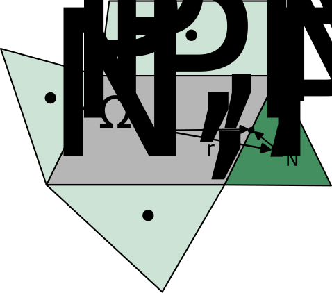
Fig. 3.1 Control volume \(P\) and neighboring cell \(N\) for integration on a 2D unstructured grid.#
Throughout this chapter, the pair \(P/N\) is used for a current cell and one specific neighbor in local two-cell derivations. In assembled-row formulas, \(\sum_f\) denotes a sum over the faces of cell \(P\), while \(\sum_{\text{nbr}}\) denotes a sum over the cell-centered neighbors of \(P\). In a few code-facing formulas, \(L/R\) is still used when the left/right face orientation is more convenient. These are just local labeling choices for the same kind of stencil, not different classes of variables.
The continuity equation above can be written in discrete form for cell \(P\) as:
where \(\Omega_P\) is the volume of cell \(P\), and the summation is over all faces \(f\) bounding control volume \(P\). The mass flux at any face is given by
where \(\vec{A}\) is the area vector computed at the face centroid.
To touch again on the high level goal of this chapter is to show how the equations are assembled into the algebraic rows of the form:
3.1. Implemented Equation Snapshots#
For a pressure-based solver like stream, two equations worth keeping in view are the generic transported-component row and the stored pressure-correction row. The generic row pattern used for one transported component, including velocity components, energy, species, and similar transport equations, is
The pressure-correction row actually sent to the linear solver is
Here \(A_{P,\text{nbr}}^{(p')}\) should be read as the stored sparse-matrix entry in row \(P\) and column \(\text{nbr}\), so the subscript pair identifies the row/column location of that neighbor coupling in the assembled linear system. With regards to these two equation forms, everything that follows in this chapter is explaining how the face fluxes, diffusion terms, momentum-interpolation choices, compressibility terms, boundary conditions, etc. feed the coefficients in those row equations.
3.1.1. Reading The Algebraic Row#
Before going term by term, it helps to fix one consistent reading of the semi-implicit row notation used throughout this chapter. For any row associated with cell \(P\),
\(P\) denotes the control volume whose row is being assembled, \(\sum_f\) denotes a sweep over the faces of that same control volume, and \(\sum_{\text{nbr}}\) denotes the immediate cell-centered neighbors that appear in the compact implicit stencil of that row. On the cell-centered unstructured meshes considered here, each interior face of cell \(P\) has one adjacent neighboring cell on the other side, so the face sum and the neighbor sum are two views of the same compact stencil: \(\sum_f\) is the natural notation during face-based flux assembly, while \(\sum_{\text{nbr}}\) is the natural notation once those face contributions have been collected into one sparse algebraic row.
For boundary-face quantities, this chapter uses the subscript \(\mathrm{bnd}\). When a sum over boundary faces of cell \(P\) is needed, the notation \(\sum_{\text{bnd}}\) is used. If only one class of boundary faces contributes, that qualifier is attached directly to the sum; for example, \(\sum_{\text{bnd}^(p)}\) denotes a sum over the specified-pressure boundary faces of cell \(P\).
That distinction is important because some approximations do use information from a wider reconstruction or gradient stencil. Those extra cells are not what nbr means in the assembled formulas of this chapter. When wider-stencil information is used, its effect is usually kept explicit and collected into source-like correction terms in \(b_P^{(\phi)}\). This is exactly why the implicit row continues to involve only the immediately adjacent neighbors of cell \(P\).
The coefficient bookkeeping is therefore additive. For a generic transported row, the final stored coefficients are built by collecting the contribution from each modeled piece:
The same bookkeeping can also be grouped more coarsely into temporal and spatial contributions:
The boxed summaries throughout this chapter are meant to be read as the pieces that are added together to form the final \(a_P^{(p')}\), \(a_{\text{nbr}}^{(p')}\), and \(b_P^{(p')}\) of the assembled row.
3.2. From Transport Equations to Algebraic Rows#
This section shows how common transport equations are turned into the algebraic cell rows used repeatedly in the solver. For the true scalar equations such as energy, species, and turbulence transport, this template applies directly. Each momentum component can also be brought into an analogous row form, but the pressure term and some viscous-stress contributions require additional treatment that will be called out explicitly rather than hidden inside the generic notation.
First, consider the common transport template as a generic scalar transport equation:
where \(\phi\) can stand for one transported component such as \(u\), \(v\), \(w\), \(H\), or \(Y_k\), \(k\), \(omega\), etc. The equation above is the common row template for a single transported unknown. The terms labeled in the equation above are:
(1) Unsteady: the time-derivative contribution.
(2) Convection: the advective flux divergence.
(3) Diffusion: the diffusive flux divergence.
(4) Source terms: any remaining contributions not captured by the above three.
For a control volume (e.g., one labeled \(P\) above), if Euler implicit time-marching scheme is employed, the discretized equation after integrating in space can be expressed in the following form:
The main components of the discretization procedure for the above equation are:
Discretization of the convection terms
Discretization of the diffusion terms
Estimation of the mass flux at control volume faces
The discretization, to be described in the following sections, leads to an algebraic equation for each control volume which can be written as:
where nbr denotes one of the immediate cell-centered neighbors of control volume \(P\). The subscript \(\mathrm{spatial}\) means that the convection, diffusion, and spatial source pieces have been collected while the transient storage term is still displayed separately. Once the new-time part of the transient term is moved into the diagonal and the known time-level part is moved to the right-hand side, the row has the compact form introduced above, with \(a_P^{(\phi)}\) as the final central coefficient, \(a_{\text{nbr}}^{(\phi)}\) as the final implicit neighbor couplings, and \(b_P^{(\phi)}\) as the final discrete source term. In the face-based assembly procedure used here, a sweep is performed over all the faces and their flux contributions are distributed to the two control volumes (cells) on either side of each face. Then, the discrete equation is constructed for the entire grid by sweeping over all the control volumes and summing up the flux contributions from all the faces.
3.2.1. Diffusion Terms#
In the generic transport equation, Eq. (3.2.1), the diffusion operator is
For one control volume \(P\), the first step is to integrate that operator over the cell volume \(\Omega_P\):
Using the divergence theorem, \(\int_{\Omega_P} \nabla \cdot (\Gamma \nabla \phi)\, d\Omega = \int_{\partial \Omega_P} \Gamma \nabla \phi \cdot \hat{\vec{n}}\, dA\), so the volume integral becomes a net diffusive flux through the cell boundary.
In the face-based finite-volume discretization used by Stream, that boundary integral is approximated by summing the flux through each face of the control volume. This is why the discrete diffusion contribution naturally appears as a face sum rather than as a cell-centered Laplacian:
Here \(D_f\) is simply a shorthand for the diffusive contribution coming through face \(f\) i.e.
To obtain implicit matrix coefficients, each face contribution must next be written in terms of the unknowns stored at the two cells adjacent to that face, namely \(P\) and \(N\).
The adjective “standard” here means the usual finite-volume decomposition used on non-orthogonal cell-centered meshes. First, introduce the center-to-center vector from cell \(P\) to cell \(N\),
Along that line, the directional derivative is approximated by the two-point difference
The motivation for using this simple approximation should be stated explicitly. At this stage of the discretization, we are trying to build an implicit matrix row with a small, local stencil: ideally one diagonal contribution for cell \(P\) and one neighbor contribution for cell \(N\) from each face. The two-point difference above does exactly that, because it depends only on the immediately adjacent cell values \(\phi_P\) and \(\phi_N\). A wider-stencil or higher-order reconstructed face gradient could certainly be used to improve the estimate of \((\nabla \phi)_f\), but if that information were kept fully implicit it would generally enlarge the stencil and complicate the matrix coefficients. The choice made here is therefore: keep the center-to-center derivative simple and local in the implicit operator, and treat the remaining non-orthogonal part as an explicit correction.
The geometric issue is that the derivative we can approximate implicitly with neighboring cell values is the derivative along \(\hat{\vec{r}}_{PN}\), while the flux we actually need is the derivative contracted with the face area vector \(\vec{A}_f\). On an orthogonal mesh those directions are aligned. On a skewed mesh they are not.
To keep the implicit part aligned with the simple \(P\)–\(N\) stencil, we write the face area vector as a decomposition into two vectors.
We define \(\vec{E}_f\) to be the part that is parallel to the vector connecting the cell centers, \(\hat{\vec{r}}_{PN}\) .
This leaves the remainder \(\vec{T}_f\) as the part of the original face area vector that is not carried by the center-to-center aligned contribution \(\vec{E}_f\).
Here, we choose what is called the over-relaxed decomposition, which means that \(\alpha_f\) is not the ordinary projection of \(\vec{A}_f\) onto \(\hat{\vec{r}}_{PN}\), but rather an over-relaxed value chosen so that the remainder \(\vec{T}_f\) is tangent to the face. The reason for that choice is that the face flux contribution from \(\vec{T}_f\) will be treated explicitly as a correction, so it is desirable to make it as small as possible by making it tangent to the face. If \(\vec{T}_f\) were not tangent to the face, then it would have a normal component that would contribute to the implicit flux and therefore feed into the matrix coefficients, which would defeat the purpose of keeping the implicit part aligned with the \(P\)–\(N\) stencil. A statement of this condition is:
We can get the value of \(\alpha_f\) that makes this condition true by substituting \(\vec{T}_f = \vec{A}_f - \alpha_f \hat{\vec{r}}_{PN}\) into that equation:
Solving for \(\alpha_f\) gives:
The decomposition of the face area vector into the aligned part \(\vec{E}_f\) and the tangential correction \(\vec{T}_f\) is therefore:
Over-Relaxed Decomposition Step
With the centerline-aligned part being \(\vec{E}_f\), and the tangential part being \(\vec{T}_f\).
With that notation, substituting Eq. (3.2.1.13) into Eq. (3.2.1.4) gives the exact split
Now the two-point approximation can be substituted directly into the directional derivative along \(\hat{\vec{r}}_{PN}\):
That covers the aligned part of the flux, but the remaining face gradient in the correction term still needs to be approximated so as to not have any unknowns at the face. The choice made here is to use a lagged face gradient \(\overline{\nabla \phi}\) that is estimated from the neighboring cell-centered gradients. This means that the correction term will be treated explicitly as part of the source term \(b_P\) rather than being fed into the matrix coefficients.
Final Scalar Diffusion Flux Split
With those two approximations, the face diffusion flux is
The first term is the compact implicit contribution built from the local \(P\)–\(N\) stencil, while the second term is the explicit non-orthogonal correction.
Assumptions In This Split
Two different approximations are being made here, and they are intentionally not the same.
For the aligned part, we use the two-point directional derivative \(\;(\nabla \phi)_f \cdot \hat{\vec{r}}_{PN} \approx (\phi_N - \phi_P)/d_{PN}\;\), because this keeps the implicit matrix contribution local to the \(P\)–\(N\) stencil.
For the correction part, we do not apply the same two-point approximation, because that difference only approximates the derivative along the center-to-center direction, not the leftover tangential direction carried by \(\vec{T}_f\). Instead, that term is treated explicitly with a lagged face-gradient estimate.
In practice, \(\overline{\nabla \phi}\) should be read as an approximation to the gradient field at the face obtained from the neighboring cell-centered gradients. In the simplest form used in this discussion,
So the second term is still approximate; it is just approximate in a different way. The first term gives the compact implicit diffusion coefficient, while the second term carries the non-orthogonal correction explicitly.
Important
When The Field Is Not Smooth The discussion above assumes that the gradient field is smooth enough that a face-gradient estimate such as \(\overline{\nabla \phi}_f\) is meaningful. When \(\phi\) has a sharp jump, when the mesh under-resolves a thin layer, or when the diffusivity changes abruptly across the face, that assumption becomes weaker and the explicit non-orthogonal correction can become noisy or overly aggressive.
Common remedies in such situations are:
reduce or suppress the non-orthogonal correction locally and rely more heavily on the compact two-point implicit term;
limit the reconstructed cell-centered gradients before forming \(\overline{\nabla \phi}_f\);
use a more appropriate face diffusivity, such as a harmonic average, when the coefficient \(\Gamma\) itself changes abruptly;
for genuine material interfaces or other true discontinuities, replace the simple averaged face-gradient model with a one-sided or interface-aware treatment.
The main point is that the compact split derived above is most reliable when the field is reasonably smooth over the \(P\)–\(N\) stencil. Near strong jumps, extra limiting or interface modeling may be needed for robustness.
If we now introduce the shorthand
then Eq. (3.2.1.16) can be rewritten in the compact coefficient form
That last line is the key algebraic step for the reader. It shows directly how the face diffusion flux has been split into a part multiplying the current-cell unknown \(\phi_P\), a part multiplying the neighbor unknown \(\phi_N\), and a remainder that is treated explicitly.
For one interior face shared by cells \(P\) and \(N\), the contribution to the row of cell \(P\) is simply
So, from this one face, the diagonal increment is \(\mathcal{K}_f^\phi\), the neighbor coefficient multiplying \(\phi_N\) is \(\mathcal{K}_f^\phi\), and the explicit source increment is \(S_{D,f}^{\mathrm{corr}}\). The full diffusive part of the cell row is obtained only after summing these facewise increments over all faces of cell \(P\) and then combining them with the transient, convective, and source contributions in Eq. (3.2.3).
Final Standard Diffusive Row Contribution
After summing the face contributions for cell \(P\) and rearranging them into the row form of Eq. (3.2.3), the diffusive part of the row is
with
and
Those are precisely the diffusion pieces that later get added into the full row coefficients \(a_P^{(\phi)}\), \(a_{\text{nbr}}^{(\phi)}\), and \(b_P^{(\phi)}\).
3.2.1.1. Additional Terms For Momentum Diffusion#
For scalar equations such as energy, species, and turbulence transport, the diffusion discussion above is the whole story: the diffusive flux is just the generic term in Eq. (3.2.1.3). The momentum equations, on the other hand, contain additional viscous-stress pieces beyond that generic scalar form. This subsection isolates those extra momentum-specific pieces. In vector/tensor form, the viscous contribution is
where \(\Gamma = \mu + \mu_t\) and \(\mathbf{I}\) is the identity tensor. Here \(\mu\) is the molecular (laminar) dynamic viscosity, while \(\mu_t\) is the turbulent or eddy viscosity supplied by the turbulence model. In a laminar calculation, \(\mu_t = 0\), so \(\Gamma\) reduces to the physical viscosity \(\mu\) alone. It is convenient to split this into a Laplacian-like part and a remaining viscous-stress correction:
After integrating over the control volume, the first term becomes
which is just the vector analogue of the generic diffusion term in Eq. (3.2.1.3), applied componentwise to the velocity field. The second term in Eq. (3.2.1.25) becomes
and is treated explicitly as part of the momentum source term. This means that \((\nabla \vec{u})_f\) and \((\nabla \cdot \vec{u})_f\) are not introduced as additional face unknowns in the implicit system. Instead, they are reconstructed from the cell-centered velocity-gradient field and then interpolated to the face in a lagged manner. At the level of this derivation, one can think of interior-face estimates such as
with the understanding that the exact interpolation and boundary treatment are implementation details. The important structural point for this section is that this second viscous term is handled explicitly from reconstructed gradients, whereas the compact \(\nabla \cdot (\Gamma \nabla \vec{u})\) part is the part kept in the local implicit stencil. When the solver assembles one momentum-component row, it simply takes the corresponding component of these vector expressions.
That means an algebraic row can be written for the diffusion part of one momentum component just as it was for a generic transported scalar. If we denote by \(u_i\) the selected velocity component, then the compact Laplacian-like part contributes exactly the same kind of local \(P\)–\(N\) coefficient as before, now with \(\phi = u_i\). The extra viscous-stress piece contributes only to the explicit source because it is reconstructed from lagged gradients rather than implicitized as additional face unknowns.
For one interior face shared by cells \(P\) and \(N\), define the explicit momentum-diffusion correction for component \(i\) by
Then the diffusive contribution from that one face to the \(i\)th momentum-component row is
where \(\mathcal{K}_f^{(u_i)}\) is the same compact coefficient defined in the generic diffusion derivation with \(\phi=u_i\), and \(S_{D,f,i}^{\mathrm{corr}}\) is the non-orthogonal correction from that same derivation, again evaluated for \(\phi=u_i\).
Final Momentum-Diffusion Row Contribution
For one velocity component \(u_i\), the diffusive part of the assembled momentum row is
with
So the bookkeeping is the same as before:
the Laplacian-like part feeds the diagonal and neighbor coefficients,
the non-orthogonal diffusion correction stays in the explicit source,
and the extra viscous-stress term also stays in the explicit source.
Important
Smoothness Caveat For The Viscous-Stress Correction This explicit viscous-stress correction inherits the same kind of smooth-field assumption as the earlier non-orthogonal diffusion correction. Its accuracy depends on the reconstructed velocity-gradient field being smooth enough that face estimates of \((\nabla \vec{u})_f\) and \((\nabla \cdot \vec{u})_f\) are meaningful.
The relevant warning sign here is a sharp variation or unresolved jump in the velocity field, if velocity or viscosity changes abruptly across a short distance, the reconstructed gradients can become noisy and the explicit correction can be too aggressive.
In such situations, the same kinds of remedies discussed above may be needed: limiting the reconstructed gradients, damping the explicit correction, or using more specialized interface-aware treatment when a true discontinuity is present.
3.2.2. Convection Terms#
We now turn to the convective face flux that appears in Eq. (3.2.3). We therefore begin at that generic level, where \(\phi\) denotes an arbitrary transported variable and the algebra applies equally to energy, species, turbulence variables, or one component of velocity. The pressure-gradient term is not part of convection, so it is handled separately in the next section.
For ease of illustration, the convection discussion below uses an upwind scheme for the transported primitive variable. When we return to the momentum-specific pressure term, we use a central-difference treatment for that separate contribution. Upwind schemes are commonly employed for incompressible flows. They can also be employed for compressible flows, though characteristics-based methods are usually more appropriate for compressible flows; those are described in a later chapter.
For cell \(P\), the discrete convection contribution that appears in Eq. (3.2.3) is the face sum
so each face contributes one term \(\dot{m}_f \phi_f\) to the cell equation. The purpose of the discussion below is to rewrite that face contribution into pieces that can be identified with the diagonal coefficient \(a_P^{(\phi)}\), the neighbor coefficient \(a_{\text{nbr}}^{(\phi)}\), and, when higher-order reconstruction is used, the explicit source term \(b_P^{(\phi)}\).
While discretizing this convection term, the mass flux \(\dot{m}_f\) is assumed to be known and is considered positive along the direction of the face normal pointing away from cell \(P\) (and towards cell \(N\)). Thus, the convective flux at any face is given by \(\dot{m}_f \phi_f\) where the face value of the transported variable \(\phi_f\) is obtained by upwinding based on the sign of the mass flux:
where \(\phi_{f,P}\) and \(\phi_{f,N}\) are the candidate face values at face \(f\) reconstructed from cells \(P\) and \(N\), respectively. In other words, the notation means “the value supplied to face \(f\) from the \(P\) side” and “the value supplied to face \(f\) from the \(N\) side.” This notation is intentionally generic: for a first-order upwind scheme, no reconstruction is used, so these reduce to the adjacent cell values \(\phi_{f,P}=\phi_P\) and \(\phi_{f,N}=\phi_N\); for a second-order upwind-type reconstruction, they are the reconstructed values obtained from the cell-centered gradients. The actual face value \(\phi_f\) is then whichever of these two candidate values lies on the upwind side of the face.
We have not used a split-flux notation earlier in the guide, so we introduce it here for convenience. Define the positive and negative parts of the face mass flux by
so that both \(\dot{m}_f^{+}\) and \(\dot{m}_f^{-}\) are nonnegative magnitudes. With these definitions, the convective face flux for a face can be written in the generic split form
This split form does not introduce a new physical model. It is simply a compact algebraic way to encode the sign-based donor-cell choice without writing a case distinction for every face. If \(\dot{m}_f>0\), then \(\dot{m}_f^{+}=\dot{m}_f\) and \(\dot{m}_f^{-}=0\), so the flux reduces to \(\dot{m}_f\phi_{f,P}\). If \(\dot{m}_f<0\), then \(\dot{m}_f^{+}=0\) and \(\dot{m}_f^{-}=-\dot{m}_f\), so the same expression reduces to \(\dot{m}_f\phi_{f,N}\).
The notation is useful because it makes matrix assembly much easier to read. Once the flux is written in split form, the coefficient multiplying \(\phi_P\) can be identified immediately as part of the diagonal contribution, while the coefficient multiplying \(\phi_N\) is the neighbor contribution.
To construct a second-order scheme, a linear reconstruction procedure is adopted for computing the candidate face values \(\phi_{f,P}\) and \(\phi_{f,N}\) by using the gradient of \(\phi\) computed at the cell centers. The gradient reconstruction operator is modified by using a limiter (\(\Psi\)) in order to avoid any local extrema. The final expressions are as follows:
where \( \vec{dr} \) is the vector from the centroid of the cell to the centroid of the face. Two limiters are used, namely, those proposed by Barth and its modification proposed by Venkatakrishnan. For cell \(P\), the Barth limiter is computed as follows:
first compute \(\phi_P^{\min}=\min(\phi_P,\phi_{\text{neighbors}})\) and \(\phi_P^{\max}=\max(\phi_P,\phi_{\text{neighbors}})\)
next, each vertex i of the cell, compute \(\phi_i\) using the equation above with \(\Psi\) set to 1.
then, compute:
finally, compute \(\Psi_P=\min(\bar{\Psi}_{Pi})\), where \(i=1,\ldots,NV_P\) and \(NV_P\) is the number of vertices in cell \(P\).
Similarly, one can compute the limiter function \(\Psi_N\) for cell \(N\). Substituting these reconstructed candidate values into the generic split-flux form gives
Separating the first-order part from the reconstruction increment gives
If we define \(\phi_f^{(1)}\) as the selected first-order face value and collect the higher-order reconstruction increment into
then the facewise convective flux can be written as
This is the key algebraic split for convection. The first term is the compact first-order upwind operator, and the second term is the reconstruction increment that upgrades that first-order face value to the selected higher-order face value. For a first-order scheme, \(\delta \phi_f^{(2)} = 0\) and only the compact upwind term remains.
Summing the facewise identity over all faces gives
For the generic transported-variable row in Eq. (3.2.3), this already shows how convection enters the algebraic form in the direct split-flux view: for one interior face \(f\), the first-order part contributes \(\dot{m}_f^{+}\) to the coefficient multiplying \(\phi_P\), contributes \(\dot{m}_f^{-}\) to the coefficient multiplying \(\phi_N\), and contributes \(-\dot{m}_f \, \delta \phi_f^{(2)}\) as an explicit source term. This correction is treated as a source term because, in the linear solve, it is evaluated from lagged reconstructed gradients and limiters rather than being implicitized as part of the compact local \(P\)–\(N\) stencil. If it were kept fully implicit, the coefficients would depend not only on \(\phi_P\) and \(\phi_N\) but also on the wider set of cells entering the reconstructed gradients and limiter values.
Final Standard Convective Row Contribution
For the direct split-flux form of Eq. (3.2.3), the convective contribution is
with
So in the direct form, the outgoing first-order flux feeds the diagonal, the incoming first-order flux feeds the neighbor coefficient, and the higher-order reconstruction increment remains explicit.
A commonly used variation of the convective discretization is to subtract \(\phi_P\) times the discrete continuity equation from the transport row. This does not change the converged equation when discrete continuity is satisfied, but it reshuffles the algebra in a way that is often helpful for diagonal dominance and linear-solver robustness. The continuity equation used here is the same cellwise balance already written in Eq. (3.3), i.e. the continuity equation after integration over control volume \(P\) and replacement of the surface integral by the face-flux sum. Written before any terms are dropped or regrouped, that operation is
We can move some terms around to get to a form that looks similar to the canonical transport template in Eq. (3.2.3):
The reason for writing it this way is that the subtracted bracket is exactly zero when discrete continuity is satisfied, so this does not change the converged equation; it only changes how the convective and unsteady pieces are arranged during the linear solve. We are not throwing away the rest of the transport row. Diffusion and other explicit source terms are untouched by this particular manipulation, because they are not part of the continuity equation. The unsteady term is also affected by the same continuity-added operation, but its bookkeeping belongs with the temporal coefficient assembly rather than with the face-by-face convection algebra. In the discussion just below, we therefore focus only on the convection part of that altered equation and how that reshuffling changes the algebraic form of the convective contribution to the row coefficients. Focusing on that second term in brackets, we see that it bears the same resemblance to the original convection term with an extra subtraction:
If continuity contains a mass source, the same idea applies, but the subtracted continuity balance must include that source. In residual form, the quantity multiplied by \(\phi_P\) is then
Thus the continuity-added manipulation remains an algebraic rewrite of the same converged equation when particle mass transfer or another mass source is active. Any apparent \(+\phi S_{\rho}\) term introduced by writing a specific-variable equation with a conservative \(\rho\phi\) left-hand side is canceled by the corresponding \(-\phi S_{\rho}\) contribution from the full continuity residual. The physical model source \(S_{\rho\phi}\) itself is not canceled. The source-aware continuum bookkeeping is summarized in the detailed governing-equations appendix.
We know how that first term can be written from (3.2.2.11), and we know the definition of the split mass flux from (3.2.2.3), so we can write the whole convection contribution in the continuity-added form as:
A little algebraic manipulation gives
The first two terms cancel, leaving
The continuity subtraction reorganizes only the first-order part. The higher-order reconstruction term \(\sum_f \dot{m}_f \, \delta \phi_f^{(2)}\) carries through unchanged.
Final Continuity-Added Convective Row Contribution
For the continuity-added form of the same transport template, the convective contribution is
with
So the continuity subtraction reshuffles only the first-order part of the convective operator: the inflow contribution becomes the implicit backbone, while the higher-order reconstruction term remains explicit in the source.
3.2.3. Pressure Contribution in the Momentum Row#
Unlike the diffusion and convection terms discussed above, pressure does not appear in the generic transported-scalar row of Eq. (3.2.3). It enters only after we specialize \(\phi\) to the momentum equation. Written in the same semi-discrete control-volume style used for the scalar transport equation, the momentum balance for cell \(P\) is
This is the vector analogue of Eq. (3.2.3): the transient and convective terms look the same in structure, the viscous contribution is gathered into the face sum \(\sum_f \vec{D}_f\), and the momentum equation carries one extra term that the generic scalar row does not, namely the pressure-gradient contribution. Here \(\vec{D}_f\) denotes the total viscous face contribution, including both the Laplacian-like diffusion part and the additional momentum-specific viscous-stress correction discussed in the previous subsection.
The pressure term we are concerned with in this section is therefore the control-volume pressure contribution. Define
This contribution can be discretized in two closely related ways. If it is treated as a volume term built from the cell-centered pressure gradient, then
In plain language, this first form says: estimate one pressure-gradient vector at the cell center, and use that single vector to represent the pressure force over the whole control volume. It does not mean that pressure is assumed constant in the cell. Rather, it means that the integrated pressure-force term is approximated from a cell-centered gradient estimate. This is the form used in the momentum relation employed for face-mass-flux construction in the next subsection.
The same contribution can also be written in surface-integral form by starting from the continuous \(-\nabla p\) term in the momentum equation and applying Green’s theorem over cell \(P\):
In this second form, the pressure contribution is viewed as the sum of the pressure forces acting on the cell faces. So the discrete data now live at the faces: one estimates a pressure value \(p_f\) on each face, multiplies by the face area vector, and sums those contributions around the control volume.
So the conceptual difference is:
Cell-centered gradient form: one gradient vector per cell, used to approximate the integrated pressure force.
Face-based form: one pressure estimate per face, used to build the integrated pressure force as a sum of face contributions.
In the continuous equations these are equivalent descriptions of the same term. Discretely, however, they are not identical, because one relies on a cell-centered gradient reconstruction while the other relies on face-pressure estimates. In both cases, it is this quantity \(\mathcal{P}_{P,i}\) that appears with a minus sign in the integrated momentum balance of Eq. (3.2.3.1).
3.2.3.1. Estimation of Mass Flux at Control Volume Faces#
We now derive the control-volume face mass-flux expression used in the pressure-coupling procedure. For a co-located arrangement of pressure and velocity components, a simple averaging of cell-centered velocities to obtain interface velocity leads to the well-known checker-boarding problem. To avoid this, a Rhie-Chow-type pressure-difference correction is introduced while computing the face mass flux [RC83].
The word “dissipation” can be misleading here, so it is worth stating explicitly what is meant. This term is not a physical viscous dissipation term and it is not meant to dissipate momentum in the same sense as viscosity. What it damps is a spurious high-frequency pressure mode on a collocated grid, namely the odd-even or checkerboard pressure pattern that can otherwise survive while producing little or no corresponding change in the naively interpolated face velocity. In that sense, it acts as a numerical pressure-mode damping term.
In the algebra below, this damping appears first as the pressure-difference-dependent part of the face mass flux in Eq. (3.2.3.30). Later, when the face-flux correction is linearized for the pressure-correction equation, the same idea appears in the generic coefficient form
So this “dissipation term” does not enter the momentum row as a separate viscous-like source. Its main algebraic role is through the face mass flux, and from there through the pressure-correction coefficients that couple neighboring pressures.
First, write the semi-discrete momentum balance in a form parallel to Eq. (3.2.3):
For the Rhie-Chow-style derivation, it is convenient to rewrite this in compact assembled form by absorbing the new-time transient contribution into the diagonal coefficient and moving the old-time transient contribution to the right-hand side. With that bookkeeping, the momentum row at cell \(P\) becomes:
Here \(a_P^{(u)}\) is the fully assembled diagonal momentum coefficient, including the implicit transient, convective, and diffusive pieces. The vector \(\vec{b}_P^{(u)}\) contains the explicit source terms together with the old-time contribution from the transient term. Thus, the velocity at cell \(P\) can be written as:
where \(\vec{H}_P\) is the non-pressure part of the assembled momentum row:
The velocity at cell \(N\) can be expressed in a similar manner:
The next step is the Rhie-Chow face-velocity construction. This is not an exact identity obtained by simple algebra alone; it is the modeling step that converts the two cell-centered momentum relations into a face-normal velocity formula suitable for a collocated grid.
The idea is:
interpolate the non-pressure quantity \(\vec{H}/a\) from the two neighboring cells to the face,
but do not obtain the face pressure effect by merely averaging the already pressure-corrected cell velocities,
instead, approximate the face-normal pressure gradient directly from the pressure difference between the two cells sharing the face.
This is the step that prevents the pressure term from disappearing too easily under naive interpolation and thereby suppresses the checkerboard pressure mode described above.
Starting from the cell-centered relations for \(\vec{u}_P\) and \(\vec{u}_N\), the Rhie-Chow prototype is obtained by projecting along the face normal and interpolating the non-pressure and pressure-response factors to the face. Before any approximation is made for the face pressure gradient itself, that prototype may be written as
Assumptions Behind This Face Form
This compact expression is a Rhie-Chow interpolation ansatz, not an exact identity like a basic algebraic rearrangement. Several modeling assumptions are built into it:
the cell-centered split \(\vec{u} = \vec{H}/a - (\Omega/a)\nabla p\) is assumed to remain meaningful when carried to the face,
the diagonal momentum coefficient \(a\) is assumed to represent the dominant local response of the momentum equation, so that \(\Omega/a\) can act as a scalar pressure-response factor,
the ratios \(\vec{H}/a\) and \(\Omega/a\) are assumed to be quantities that can be interpolated to the face independently,
and the face-normal velocity is assumed to be well represented by projecting that interpolated split onto \(\hat{\vec{n}}_f\).
So this step should be read as the chosen collocated-grid face model used for pressure-velocity coupling, not as something that follows from first principles without approximation.
In this notation, \(a\) is not a new standalone variable. At the cell centers it is just the diagonal momentum coefficient, namely \(a_P^{(u)}\) or \(a_N^{(u)}\). At the face, quantities such as \((\vec{H}/a)_f\) and \((\Omega/a)_f\) mean the corresponding cell-centered ratios interpolated to the face.
The remaining modeling step is to approximate the face-normal pressure gradient by the two-point center-to-center formula [FP02]:
Substituting that approximation into the previous expression gives the familiar Rhie-Chow face-normal velocity form
For the present derivation, these face-interpolated factors are first approximated by simple arithmetic averages:
This is the equal-weight midpoint form of the interpolation. In the code-facing formulas, however, stream usually writes these face values with a geometric interpolation factor based on the distances from the face center to the neighboring cell centers:
so that the same face quantities are written as
Equivalently, one may write a generic face weight \(\lambda_f\) as
with a similar expression for \((\Omega/a)_f\). In the notation used by the implementation, \(\lambda_f=1-I\). The equal-weight midpoint form used below is therefore recovered when \(I=\tfrac{1}{2}\). Keeping the prototype in midpoint form makes the Rhie-Chow algebra a little easier to read, but the reader should recognize that the implemented MI_OldForm replaces those \(\tfrac{1}{2}\) averages by geometric weights \(I\) and \(1-I\).
The first principle used to pass from face velocity to face mass flux is simply the definition
Substituting Eq. (3.2.3.13) into that definition gives the intermediate Rhie-Chow mass-flux form
At this stage, the goal is very concrete: every quantity in this face mass flux must be replaced by an explicit face model built from the neighboring cell data. In practice, that means we still need usable expressions for
the transport-like face term \(\left( \vec{H}/a \right)_f \cdot \hat{\vec{n}}_f\),
and the pressure-response factor \(\left( \Omega/a \right)_f\).
The remaining step is another approximation, not a new conservation law. The key issue is that the mass flux is a face quantity, but the momentum relations we actually know are written at the two neighboring cell centers. So this step is doing two distinct things:
first, it uses the two cell-centered momentum relations to build a face estimate for the interpolated non-pressure quantity \((\vec{H}/a)_f \cdot \hat{\vec{n}}_f\);
second, it replaces the resulting average of two cell-centered pressure-response terms by a more compact face model involving one face coefficient \((\Omega/a)_f\) and one face-gradient estimate.
The first part explains why an average appears at all: it is simply the midpoint face interpolation of information known only at cells \(P\) and \(N\).
This is also the point where the usual Rhie-Chow “pseudovelocity” interpretation is helpful. If we define
then the cell-centered momentum relations read
Equivalently,
The Rhie-Chow idea is then: interpolate the pseudovelocity to the face, but evaluate the pressure derivative directly at the face. In other words, it amounts to adding and subtracting pressure-derivative contributions evaluated at different locations.
Averaging those two identities and taking the face-normal component gives
Up to this point, nothing new has been assumed. But this averaged identity still contains an awkward term:
which is an average of two cell-centered pressure-response contributions. That is not yet the compact face form used in the Rhie-Chow mass flux. The extra modeling step is therefore:
identify the left-hand side with the interpolated face quantity \((\vec{H}/a)_f\cdot \hat{\vec{n}}_f\),
and replace the averaged cell-centered pressure-response term by a face-interpolated coefficient multiplied by a face-gradient estimate projected along the center-to-center direction.
If we denote the chosen face interpolation of the pressure-response factor by
then this gives
and therefore the compact face model
So the main idea is: start from the centered transport velocity, then add back a face-model estimate of the pressure contribution already contained in the neighboring cell velocities.
Now do the substitution literally in the intermediate mass-flux form:
The same face pressure-response factor multiplies both pressure-related pieces, so those two terms can be grouped together:
That regrouping is exactly where the bracketed correction comes from: it is not introduced separately, but appears when the directly evaluated face-pressure term and the pressure contribution already embedded in the interpolated neighboring velocities are collected under the same face coefficient. Writing the result compactly gives the commonly used corrected mass-flux expression:
Here the overbar on \(\overline{(\Omega/a)}_f\) means that the ratio \(\Omega/a\) itself is interpolated to the face. That is the quantity naturally produced by the cell-centered momentum relations and it is also the quantity directly interpolated in the implementation. Writing the term instead as \((\rho A \Omega)_f\,\overline{(1/a)}_f\) would introduce one more factorization approximation, namely replacing a face interpolation of the ratio by the product of separately interpolated factors. That may be reasonable on smooth meshes, but it is not the clearest way to present the Rhie-Chow prototype here.
So the bracketed term should be read as the mismatch between:
the two-point pressure difference across the face, and
the pressure difference that would be predicted from the interpolated cell-centered pressure gradient.
Equivalently, in the language often used in Rhie-Chow derivations, it is the face pressure derivative minus the average of the pressure derivatives implied by the neighboring cell-centered momentum equations. This is why the correction vanishes for a locally linear pressure field and only acts when those two pressure-derivative estimates do not match. In Eq. (3.2.3.30), \(\vec{u}\) is the velocity field that satisfies the momentum equations during the sequential solution procedure, \(\overline{(\Omega/a)}_f\) is the face interpolation of the local pressure-response factor, and \(\overline{\nabla p}\) is the volume-weighted average of the adjacent cell-centered pressure gradients. Note that the interface density \(\rho_f\) is obtained by averaging (for incompressible flows) or upwinding (for compressible flows) the adjacent cell values. The mass flux at a boundary face is:
where \(\rho_{\mathrm{bnd}}\) and \(\vec{u}_{\mathrm{bnd}}\) are obtained from boundary conditions, to be discussed in later sections.
The mass flux in Eq. (3.2.3.30) is, in its classical form, affected by the velocity under-relaxation used in the segregated iteration. The treatment suggested by [Maj88] removes that spurious dependence. To show the idea, write the under-relaxed version of Eq. (3.2.3.8) as
where \(\alpha\) is the velocity under-relaxation factor and the superscript \(\mathrm{old}\) denotes the value from the previous nonlinear iteration. Using the analogous face-normal relation then leads to the Majumdar-corrected mass-flux prototype below.
Equation (3.2.3.33) is the canonical structure to keep in view for the Rhie-Chow-derived momentum-interpolation family. The MI_OldForm implementation is the closest direct realization of this prototype. In the code, the simple midpoint averages shown here are replaced by geometric interpolation weights \(I=d_{Pf}/(d_{Pf}+d_{Nf})\) and \(1-I\), and the newer Choi/Pascau-style forms further modify the pressure-response factor with \(\delta\)-type consistency terms coming from the unsteady momentum equation. Optional conservative variants also replace the cell-centered \(\nabla p\) contribution by the exact discrete pressure source term used in the momentum assembly.
Classical Rhie-Chow/Majumdar Prototype
The estimation of the mass flux at cell interfaces using Eq. (3.2.3.33) provides the pressure-velocity coupling needed to suppress collocated-grid pressure oscillations. On uniform meshes this effect is commonly interpreted as a higher-order pressure-mode damping term, but the essential point here is simply that the correction removes the checkerboard mode without changing the target continuum equations.
3.2.3.2. Momentum-Interpolation Variants#
Equation (3.2.3.33) is the basic prototype behind the momentum-interpolation ideas used in stream. At a high level, all of the implemented forms may be viewed as writing the face mass flux as
where \(\dot{m}_{f,\mathrm{centered}}\) is the interpolated transport part, \(D_f \left( p_N - p_P \right)\) is the pressure-difference dissipation that suppresses checkerboarding, and \(C_f\) collects additional terms needed to make the face flux consistent with under-relaxation, time discretization, and other momentum-equation source terms.
In stream, the available momentum-interpolation forms fall into two main conceptual families.
3.2.3.2.1. Rhie-Chow / Majumdar / Pascau Family#
The first family starts from the classical Rhie-Chow idea: interpolate a velocity-like quantity to the face and then replace the face pressure gradient by a pressure difference between the two cells straddling the face. The Majumdar correction removes the spurious dependence of the dissipation term on velocity under-relaxation. This is the core idea behind the original form and it is also the starting point for the Choi and Pascau-type variants.
The main differences among these variants are not in the basic purpose of the method, but in how the correction term is made consistent with the unsteady momentum equation. In particular, the Choi and Pascau forms modify the interpolation so that the strength of the coupling does not collapse as the time step becomes small. The newer Pascau-style variants further reorganize the explicit unsteady contribution so that the mass-flux correction remains compatible with source terms such as buoyancy and acceleration terms in problems where exact cancellation is important, such as free-fall-type limits.
Within this family, stream also allows the pressure part of the dissipation to be written using the discrete pressure source term that actually appears in the momentum equation rather than only the cell-centered pressure gradients. Conceptually, this is a compatibility correction: it makes the momentum interpolation vanish exactly for uniform-flow states when the discrete momentum equation itself has that property.
3.2.3.2.2. Denner Family#
The second family is the Denner-style momentum interpolation. It still serves the same purpose, namely constructing a face mass flux that prevents pressure-velocity decoupling on a collocated grid, but it is built around a somewhat different geometric picture. Instead of expressing the correction only in terms of the face normal and a cell-centered pressure-gradient subtraction, the Denner form is written along the line connecting neighboring cell centers and uses interpolation factors based on the projected face position between those cells.
This leads naturally to a face coefficient built from the local momentum diagonals and the local density, and it allows the pressure, buoyancy, and other momentum-source contributions to be treated with the same interpolation geometry. In practice, this makes the method a distinct alternative to the Rhie-Chow/Pascau family rather than merely another small variant of it. The Denner implementation in stream also includes optional skewness corrections and higher-order pressure reconstruction terms for cases where mesh geometry plays a larger role in the face-flux construction.
The important point is that stream does not have many unrelated momentum-interpolation methods. It has one broad Rhie-Chow-derived family with several consistency refinements, and one Denner-style family that uses a different geometric construction for the face correction.
3.3. From Continuity Defect to Pressure-Correction Row#
This section plays the same role for pressure correction that the previous sections played for the transported equations: start from the semi-discrete balance for one cell, expose the individual time and face contributions, linearize the unknown correction terms, and then collect everything into one algebraic row. The focus is still assembly.
In the algorithmic roadmap of Chapter 2, this is the stage after the momentum predictor has supplied provisional face fluxes and before the pressure, velocity, and face-flux corrections are applied. Put differently, this section is where the continuity balance is rewritten into the linear pressure-correction row for \(p^{'}\).
Seen through the chapter’s repeating pattern, three ingredients have to be made explicit:
the unsteady density contribution,
the pressure-induced face-flux correction,
the bookkeeping that sends each face contribution into the diagonal, neighbor, and right-hand-side entries.
The goal is to end with the same standard assembled form that will later be mapped to pPrime_D, pPrime_L / pPrime_U, and pPrime_B.
3.3.1. State Labels and Continuity Balance#
Before breaking down the terms, fix the state labels used throughout this section. The superscript \(n\) denotes the previous converged time level. The superscript \(k\) denotes the current outer-iteration estimate at the new time level, and \(k+1\) denotes the next corrected estimate at that same time level. A superscript \(*\) denotes a provisional quantity available after the momentum predictor built from the current iterate. A prime denotes the correction solved for during the pressure-correction step. For pressure specifically, one may read \(p^* \equiv p^k\), whereas \(\vec{u}^*\) and \(\hat{m}_f^*\) are newly predicted provisional quantities constructed from that iterate. These symbols therefore label stages of the segregated solution procedure inside one time step; they should not be read as additional time-discretization levels. Once the outer iterations converge, the final \(k\)-state is identified with the new time level \(n+1\).
With that goal in mind, begin from the semi-discrete continuity balance for one cell after the momentum solve but before the pressure correction update. At any given outer iteration of the segregated pressure-based method, the provisional face fluxes do not, in general, satisfy discrete continuity. Let \(\hat{m}_f^{*}\) denote the predicted face flux appearing in the selected continuity form. In the ordinary mass-based form this is simply the predicted face mass flux \(\dot{m}_f^{*}\); in normalized or moving-grid forms it is the corresponding predicted flux after the appropriate normalization or geometric correction has been applied. The pressure-correction step therefore seeks a face correction, \(\dot{m}_f^{'}\), such that the cellwise continuity balance is satisfied:
This equation is the starting continuity balance for the pressure-correction derivation. It is not yet the final pressure-correction equation solved by the linear solver. The job of the next few subsections is to rewrite the unknown pieces of this balance in terms of the pressure correction \(p^{'}\): first the unsteady density term, then the face-flux correction. Once those replacements have been made, the resulting equation is collected into the standard algebraic row for \(p^{'}\).
3.3.2. Unsteady Density Contribution#
For compressible branches, the unsteady term contains the density correction. In the same spirit as the earlier transport-equation derivations, we keep the time-discrete term explicit and then split it into an unknown correction part plus a known lagged remainder:
where \(k+1\) denotes the next outer iteration at the current time level, \(k\) denotes the current corrected iterate at that same time level, and \(n\) denotes the previous converged time level.
In that sense, \(\rho_P^{'}\) is the density correction only relative to the current iterate: it is the increment that moves the new-time estimate from \(\rho_P^k\) to \(\rho_P^{k+1}\) during this pressure-correction step. It is not the full time-step change from \(\rho_P^n\) to the final converged \(\rho_P^{n+1}\).
Thus the unsteady contribution in the cell balance becomes
At this point the only unknown part of the unsteady term is the increment \(\rho_P'\). To close that term, the pressure-correction equation needs a local relation between density change and pressure change.
One way to expose the assumption is to write the thermodynamic closure in primitive form,
A first-order increment about the current nonlinear state would then contain all of the pressure, temperature, and composition sensitivities:
This is the fully coupled linearized picture. A segregated pressure-correction solve does not solve for all of these increments at once. It keeps one pressure-sensitive density response implicit in the pressure equation, while the remaining thermodynamic and composition changes are supplied by the current iterate or by later scalar / EOS updates.
Density-Linearization Assumption
If temperature and composition are lagged during the pressure-correction solve, then \(T_P'\) and \(Y_{i,P}'\) are not unknowns in that linear system. The density correction reduces to the familiar scalar form
The precise meaning of \(\psi_P\) depends on which thermodynamic tangent is chosen. The compressible pressure-correction row used here takes this pressure-density slope to be the EOS-compatible acoustic derivative, so \(\psi_P=(\partial\rho/\partial p)_{s,Y}=1/a_{s,P}^2\), rather than the isothermal slope \((\partial\rho/\partial p)_{T,Y}\).
To fix the reference-state notation for the implemented acoustic form, define
Then the first-order Taylor expansion of the EOS about the current iterate is
For the EOS linearization, that same increment is measured relative to the current-iterate reference state:
During this pressure-correction step, the remaining thermodynamic / composition state is treated as frozen at the current iterate, so only the pressure-induced part of the density response is being linearized implicitly.
The role of \(s\) here is only to identify the acoustic EOS derivative. We are not solving an entropy equation inside the pressure-correction step, and we are not assuming that the full flow is globally isentropic. The point is simply that the sound speed is defined by the isentropic tangent to the EOS, so the compatible density-pressure slope is the acoustic compressibility:
Hence the relation being used is
This is a general EOS-based thermodynamic relation evaluated with the acoustic derivative. It is therefore EOS-generic, but it is not the same as choosing some other slope such as \((\partial \rho/\partial p)_{T,Y}\) or \((\partial \rho/\partial p)_{h,Y}\).
Substituting that linearization into the unsteady term shows how the original unsteady density term in Eq. (3.3.1.1) is replaced inside the pressure-correction derivation. In other words, when we return to the starting continuity balance, the left-hand unsteady term there is replaced by the right-hand expression below. This is still only one ingredient of the derivation, not yet the final assembled pressure-correction row.
Final Unsteady Density Contribution
For the compressible pressure-correction row, the unsteady density contribution is
with
That is, the acoustic density response contributes an implicit diagonal term, while the lagged time-level defect remains on the right-hand side.
The approximation enters in using that local acoustic derivative to linearize the density change within one pressure-correction solve. In other words, this step models the pressure-induced part of the density update, not the entire density change that may occur over a full nonlinear iteration when temperature, species, phase fractions, or other closure variables also change.
3.3.3. Splitting the Face Flux#
The same predictor/corrector split is now applied to the face flux itself. Write the corrected face flux as
where \(\hat{m}_f^{*}\) is the known provisional face flux available after the momentum predictor, and \(\dot{m}_f^{'}\) is the unknown pressure-induced change in that face flux. In other words, \(\dot{m}_f^{'}\) is the amount by which the provisional face flux must change during the pressure-correction step in order for continuity to be satisfied.
To obtain a prototype expression for \(\dot{m}_f^{'}\), insert the pressure decomposition \(p=p^*+p'\) into Eq. (3.2.3.30) and collect every term involving only starred / already known quantities into \(\hat{m}_f^{*}\). The remaining term, linear in the pressure correction, is by definition the face-flux correction. This is intentionally a reduced prototype: the earlier full face-flux model contained transport and gradient-reconstruction pieces, but by this stage those known contributions have already been absorbed into \(\hat{m}_f^{*}\). For an interior face \(f\) between cells \(P\) and \(N\), the remaining pressure-correction part is therefore written in the generic coefficient form
for the basic midpoint Rhie-Chow prototype. More elaborate momentum-interpolation variants modify the precise definition of \(d_f\), but they preserve the same linear dependence on the pressure-correction difference across the face. That linear dependence is what later becomes the face coefficient in the assembled pressure-correction row.
3.3.4. Assembling One Cell Row#
At this point, the unknown pieces of Eq. (3.3.1.1) have been rewritten in terms of \(p^{'}\): the unsteady density term has been linearized, and the face-flux correction has been expressed as a pressure-correction contribution. The next step is therefore just bookkeeping: substitute those replacements back into the starting continuity balance and collect the resulting diagonal, neighbor, and source terms into the algebraic pressure-correction row.
The most useful algebraic step is to stop treating Eq. (3.3.3.2) as one compact expression and instead expand what one face contributes to the row of one cell.
For an interior face between cells \(P\) and \(N\), expand Eq. (3.3.3.2) as
where \(d_f\) is the face pressure-correction coefficient determined by the selected momentum-interpolation formula. Expanding the bracket gives
This is the key bookkeeping step. For the row associated with cell \(P\):
the term multiplying \(p_P^{'}\) contributes to the diagonal,
the term multiplying \(p_N^{'}\) contributes to the neighbor coupling.
At a specified-pressure boundary the same idea becomes one-sided. Because the boundary pressure correction is known and equal to zero, such a face contributes to the diagonal of the row for cell \(P\) but not to a neighbor coefficient. In the formulas below, the face sum \(\sum_f\) is therefore understood in the simple bookkeeping sense used throughout this section: it runs over the faces whose flux correction contributes to the pressure-correction row.
Substituting the unsteady split and the face-flux corrections into Eq. (3.3.1.1) gives us the row equation form for cell \(P\). For reference, this is the equation we will be substituting terms into.
Substituting the unsteady split and the face-flux correction gives:
where \(f\) denotes the faces of cell \(P\). The first face sum is the known provisional-flux contribution, and the second is the face pressure-difference coupling. On an interior face, \(p_N'\) is the pressure correction in the neighboring cell across that face. On a specified-pressure boundary, the boundary pressure correction is known, so only the diagonal part contributes.
All terms involving \(p_P^{'}\) can then be grouped together, with everything else moved to the right-hand side:
This is the algebra behind the statement that several different \(p^{'}\) terms are “collected into the diagonal.” The face coefficients are still indexed by face in the grouped equation above. Once those face contributions are collected into the compact row, the corresponding neighbor coefficient is simply the coefficient on the face shared by cell \(P\) and that neighbor.
Final Standard Pressure-Correction Row
For each cell \(P\), the assembled pressure-correction equation is
with
Here \(\sum_f d_f\) is the diagonal contribution from the faces that participate in the pressure-correction row. Interior faces contribute both diagonal and neighbor terms, while a specified-pressure boundary contributes only its diagonal piece. For the simple boundary treatment just derived, \(b_{P,\mathrm{bc}}^{(p')}=0\).
In incompressible branches these are already the final coefficients. In compressible branches, the upwind acoustic density correction adds extra terms to the diagonal of the upwind row and to the neighbor coefficient of the downwind row, as described next.
The base row is now in hand. The remaining subsections answer two practical follow-up questions: what extra term appears in compressible branches, and how the implementation turns the abstract coefficients above into the stored matrix row.
The previous derivation was not only for incompressible flow. It derived the base pressure-difference part of the face-flux correction, namely the term \(-d_f\left(p_N'-p_P'\right)\), which is present in both incompressible and compressible branches. In incompressible branches that base term is already the whole correction, because there is no density correction. In compressible branches, however, the pressure-correction step also changes the density, and that changing density is carried by the provisional face-normal velocity. The subsection below is therefore adding the extra compressible contribution, not replacing the derivation above.
3.3.5. Additional Compressible Density-Correction Term at Faces#
For compressible flows, the face mass-flux correction contains the same base pressure-difference term derived above, plus one additional contribution: the density correction carried by the provisional face-normal velocity. In other words, the previous subsection already supplied the \(-d_f\left(p_N'-p_P'\right)\) part; the only new ingredient here is the \(\rho_f' u_{n,f}^* A_f\) term:
At the face, the density correction is linearized with the upwind acoustic derivative,
so that the extra face term becomes
Final Compressible Coefficient Update
For the additional compressible density-correction term, the assembled-row contribution is
with
So, in compressible branches, the assembled coefficients are
So the compressible term does not introduce a new base coefficient family. It simply adds an extra contribution to the same diagonal, neighbor, and right-hand-side quantities already derived above.
This closes the generic assembled-row description. The later sparse-row subsection does not introduce a new pressure-correction equation; it only rewrites these same additions in the sign convention used by the linear solver storage.
3.3.6. Computing the Face Coupling Coefficient \(d_f\)#
The previous subsections stopped at the generic assembled row. The remaining question is therefore how the abstract face coefficient \(d_f\) is computed for a selected momentum-interpolation variant. Once that coefficient has been defined, the later collection into \(a_P^{(p')}\), \(a_{\text{nbr}}^{(p')}\), and \(b_P^{(p')}\) is unchanged.
3.3.6.1. Example: Denner Interior and Boundary Coefficients#
For the Denner-style momentum interpolation used in MI_Denner, the interior-face coefficient can be written in the form
where
and
Here \(\lambda_0\) is the first implicit time-integration coefficient (timeIntegratorFactor0 in the implementation), \(\alpha_v\) is the velocity-relaxation factor, and \(\beta_f\) is the optional skewness correction factor. In words:
start from the momentum diagonal,
subtract the implicit transient contribution to obtain the non-temporal diagonal \(\tilde a\),
form a volume-over-diagonal quantity \(\mathcal{D}_f\),
fold in the unsteady face-density correction through \(F_f=\mathcal{D}_f/(1+c_f\mathcal{D}_f)\),
multiply by density, relaxation, geometric projection, and face area to obtain \(d_f\).
That sequence is exactly what the MI_Denner interior-face rule is doing, just in code form.
At a boundary face the derivation is the same, except that there is only one adjacent cell. The Denner boundary coefficient is therefore
with
This is the algebraic answer to the question “what is the pressure-correction coefficient on a boundary face?” For a specified-pressure boundary, that \(d_{\mathrm{bnd}}\) then enters the cell equation only through the diagonal term \(d_{\mathrm{bnd}} p_P^{'}\). For a boundary where the mass flux is prescribed, no unknown pressure correction is used to alter the flux, so there is no corresponding pressure-correction coefficient in the matrix row.
The older Rhie-Chow/Pascau-style variants follow the same assembly logic after this point. What changes is the formula for \(d_f\): the Denner factors \(F_f\) and \(\beta_f\) are replaced by the appropriate diffusion-product and time-consistency factors for the selected momentum-interpolation form. Once the flux correction has been reduced to a coefficient multiplying \(p_N^{'}-p_P^{'}\), however, the later collection into \(a_P^{(p')}\), \(a_{\text{nbr}}^{(p')}\), and \(b_P^{(p')}\) is exactly the same.
3.3.7. From Assembled Coefficients to the Stored Solver Row#
The pressure-correction derivation is complete by this point. The purpose of the final subsection is not to derive a different equation, but to explain how the already assembled coefficients are stored and accumulated in the linear solver. The same \(a_P^{(p')}\), \(a_{\text{nbr}}^{(p')}\), and \(b_P^{(p')}\) contributions are still present; only the sign convention and storage layout change.
3.3.7.1. Stored Sign Convention and Temporary Accumulation#
The derivation above writes the pressure-correction equation in the usual Patankar form,
with positive neighbor coefficients \(a_{\text{nbr}}^{(p')}\). The implementation stores the same equation with the neighbor signs already absorbed into the sparse off-diagonal entries. For a cell \(P\), the row sent to the linear solver is therefore better written as
where \(D_P^{(p')}\) is the diagonal entry, \(A_{P,\text{nbr}}^{(p')} \le 0\) are the stored off-diagonal entries, and \(B_P^{(p')}\) is the right-hand side. The subscript pair on \(A_{P,\text{nbr}}^{(p')}\) is therefore a row/column index pair: row \(P\), column \(\text{nbr}\). In the implementation these correspond to the stores pPrime_D, pPrime_L / pPrime_U, and pPrime_B, respectively. Thus, relative to Eq. (3.3.4.6),
This sign change is the first source of confusion when reading the assembly rules. The second is that the code first accumulates contributions into temporary stores such as pPrimeTemp_D and pPrimeTemp_B and only later copies them into the final sparse row. The many unit/apply rules are therefore not separate equations; they are separate additions to the same final row.
3.3.7.2. Interior-Face Storage Pattern#
The numerous face-coefficient rules should be read in the same spirit. They do not define different matrix structures. They all compute the same abstract face coefficient \(d_f\), although the implementation names that quantity pPrimeCoefficient. Different momentum-interpolation variants simply provide different formulas for \(d_f\). Once \(d_f\) has been computed, the storage pattern is unchanged.
For a compact description of that pattern, define
where \(\alpha_v\) is the velocity relaxation factor and \(\delta_f\) is the face-interpolated transient correction factor used by SIMPLEC.
For the selected continuity form, let \(\tau_L\) and \(\tau_R\) denote the density-scaling factors applied when the pressure-difference coupling is inserted into the left and right cell rows. In simple mass-based forms these are just unity; in normalized variable-density forms they contain the corresponding local density normalization. The implementation controls those choices through options such as pPrimeFactor or rhoNormFactor, but the algebra below does not depend on the particular parameterization. For an interior face \(f\) between cells \(L\) and \(R\), define
These are not new physical coefficients; they are just the left-row and right-row versions of the same pressure-difference face coupling after whatever local density scaling the selected formulation uses. The stored interior-face contributions are therefore
This is the stored-row version of the same algebra already summarized in the assembled-row discussion. In particular, the SIMPLEC modification does not create a different pressure equation; it simply scales the face coupling by the factor \(1+\kappa_f\).
3.3.7.3. Compressible Additions in the Stored Row#
This subsection is still not deriving a new pressure equation. It is only translating the extra compressible coefficient update from Eq. (3.3.5.5) into the stored-row notation above.
Let \(c_f\) denote the same upwind acoustic face coefficient introduced in Eq. (3.3.5.1), after any branch-specific scaling factors have been absorbed into it. Using the same row-normalization factors \(\tau_L\) and \(\tau_R\) as above, define
Then the additional stored-row contributions are
So the storage rule mirrors the assembled-row statement exactly: the extra compressible contribution is added to the diagonal of the upwind row and to the off-diagonal entry of the downwind row. When the mesh moves, the implementation evaluates the upwind direction using the flux relative to the grid motion; in the code this relative flux is formed from volFluxStar - gridVolFlux. The implementation also folds branch-specific scaling choices, such as compressiblePPrimeFactor, into the coefficient \(c_f\).
3.3.7.4. Right-Hand-Side Assembly#
The right-hand side is assembled in the same additive way. Let \(\tau_P\) denote the local row-normalization factor for cell \(P\), consistent with the left/right factors introduced above. Then the stored right-hand side can be written as
where \(\hat{m}_f^{*}\) denotes the predicted face mass flux appearing in the selected form of the continuity equation. For a fixed grid this is simply built from the starred face flux. For moving-grid or normalized volumetric forms, the implementation instead uses the corresponding flux relative to the grid motion; this is where gridVolFlux enters the bookkeeping.
For first-order BDF in the compressible form, the explicit unsteady contribution added to the right-hand side is
For BDF2, the code adds the same first-order defect plus the lagged second-order correction, giving
where the coefficients \(c_2\), \(c_{F0}\), \(c_{F1}\), and \(c_{F2}\) are the time-integration weights introduced in Chapter 5; in the code these appear as the timeIntegratorFactor* values. In other words, the time scheme enters the final pressure-correction row in two places:
through the face coefficient \(d_f\),
through the explicit unsteady part of the right-hand side and the implicit acoustic diagonal contribution.
3.3.7.5. Boundary Summary and Code Landmarks#
Finally, boundary-specific rules are just one-sided versions of the same assembly logic. A specified-pressure boundary contributes only to the adjacent cell diagonal and right-hand side, a total-pressure inlet uses a specialized boundary coefficient, and the fixed-pressure reference cell is anchored by zeroing the appropriate source/off-diagonal entries. Reading the code this way turns the long list of apply rules into a bookkeeping exercise: each rule is simply adding one physically identifiable term to the same final linear system row.
If you want to look those objects up in the source, the most important math-to-code identifications are:
pPrimeCoefficient\(\leftrightarrow d_f\)pPrimeCoefficientTotalPressureInlet\(\leftrightarrow\) specialized boundary coefficient \(d_{\mathrm{bnd}}\)pPrimeTemp_D\(\leftrightarrow\) accumulator for the diagonal \(a_P^{(p')}\) before copy topPrime_DpPrime_L/pPrime_U/pPrime_I\(\leftrightarrow\) stored off-diagonals \(A_{P,\text{nbr}}^{(p')}\)pPrimeTemp_B\(\leftrightarrow\) accumulator for the right-hand side \(b_P^{(p')}\) before copy topPrime_B
At this point the pressure-correction equation has been fully assembled, interpreted, and translated into the solver’s storage convention. The next step is therefore not further assembly, but applying the solved correction field to the flow variables.
3.4. Applying the Pressure Correction#
Once the pressure correction field is computed by solving Eq. (3.3.4.6), the mass flux, pressure, and velocity fields are corrected schematically as follows. These are the generic corrected-state relations; the exact stored/code-level forms still depend on the selected pressure-correction variant and normalization choices discussed above.
where \(\dot{m}_f^{'}\) is given by Eq. (3.3.3.2) or Eq. (3.3.5.1). In these update equations, \(p^*\) is the pressure reference used to form \(p'\), while \(\vec{u}^*\) and \(\hat{m}_f^*\) are predicted quantities built from that reference state. \(\alpha_p\) is the under-relaxation factor for pressure, and \(a_P^{(u)}\) is the central coefficient of the momentum equations in cell \(P\). Variables with subscript \(P\) are cell-centered and those with subscript \(f\) are face-centered.
3.5. Boundary Conditions#
The different types of boundaries commonly encountered in a computational domain can be classified as: inflow, outflow, wall and symmetry boundaries. The boundary conditions are imposed in terms of the primitive variables, either by assigning them fixed values or extrapolating from the interior of the domain, depending on the local flow regime. Once the appropriate boundary mass fluxes are computed from boundary density and velocity components, the contribution to the discretized momentum and energy equations by the boundary faces is no different than any interior face. The contributions to the coefficients of the pressure correction equation, however, depend on the type of boundary, as discussed below.
At wall boundaries, the fluid velocity is the same as that of the wall which can be stationary or moving; the mass flux is zero. At symmetry boundaries, the flow is parallel to the boundary; thus, all the variables are extrapolated from the interior and the mass flux is set to zero. The inflow and outflow boundaries need special treatment depending on the flow regime and are discussed below.
3.5.1. Inlet: Fixed Mass Flux#
At an inlet, a mass flux and the flow angle can be specified. Static or total temperature is specified. Pressure can be specified or extrapolated from the interior depending on the flow regime. Three flow regimes can exist:
Constant density flow: density and velocity components are fixed. Pressure is extrapolated from the interior.
Subsonic flow: density is not fixed at the inlet. Pressure is extrapolated from the interior cells and then density is computed from the equation of state using the boundary temperature. Velocity components are then computed from the specified mass flux and flow angle.
Supersonic flow: density, velocity components and pressure are all fixed.
In all of the above situations, the mass flux at a boundary face is given by
which goes into the pressure correction equation as a source term. The mass flux correction is zero; therefore, the contribution from the boundary face to the diagonal and neighbor coefficients of the pressure correction equation given by Eq. (3.3.4.6), is also zero. It should be noted that the contribution from \(\rho^{'}\) for compressible flows, given by Eq. (3.3.5.5) is also zero for a fixed mass flux boundary.
3.5.2. Outlet: Fixed or Extrapolated Pressure#
At outflow boundaries, the velocity vector \(\vec{u}_{\mathrm{bnd}}\) is extrapolated from the interior and temperature is extrapolated. Pressure can be specified or extrapolated depending on the flow regime. Density is extrapolated from the interior. Mass flux is given by Eq. (3.5.1.1) and the mass flux correction can be written as:
The normal velocity correction at the boundary in terms of pressure correction at the boundary and the adjacent cell, analogous to correction at an interior face given by Eq. (3.3.3.2), can be written as:
Two situations can arise at an outlet:
Fixed Pressure Outlet: If the flow at the outlet is incompressible or subsonic, the static pressure is fixed which implies \(p_{\mathrm{bnd}}^{'} = 0\) .
Extrapolated Pressure Outlet: If the flow is supersonic at the outlet, then the pressure is extrapolated from the interior which implies \(p_{\mathrm{bnd}}^{'} = p_P^{'}\) .
For both of the above situations, the density correction is non-zero for compressible flows. To stay consistent with the EOS-generic acoustic linearization used throughout this chapter, we write the extrapolated boundary density correction as
and the mass flux correction is given by:
The contributions to the pressure-correction equation from outflow boundary faces are obtained directly from Eq. (3.5.2.4). If one later specializes to an ideal-gas EOS, the acoustic derivative above reduces to the familiar ideal-gas expression, but that specialization is no longer assumed implicitly here.
3.6. References#
J.H. Ferziger and M. Peric. Computational Methods for Fluid Dynamics. Springer, 3rd edition, 2002.
S. Majumdar. Role of underrelaxation in momentum interpolation for calculation of flow with nonstaggered grids. Numerical Heat Transfer, 13:125–132, 1988.
C.L. Rhie and W.L. Chow. A numerical study of the turbulent flow past an isolated airfoil with trailing edge separation. AIAA Journal, 21:1525–1532, 1983.